See any bugs/typos/confusing explanations? Open a GitHub issue. You can also comment below

★ See also the PDF version of this chapter (better formatting/references) ★

Modeling randomized computation

Formal definition of probabilistic polynomial time: the class \(\mathbf{BPP}\).
Proof that every function in \(\mathbf{BPP}\) can be computed by \(poly(n)\)-sized NAND-CIRC programs/circuits.
Relations between \(\mathbf{BPP}\) and \(\mathbf{NP}\).
Pseudorandom generators

“Any one who considers arithmetical methods of producing random digits is, of course, in a state of sin.” John von Neumann, 1951.

So far we have described randomized algorithms in an informal way, assuming that an operation such as “pick a string \(x\in \{0,1\}^n\)” can be done efficiently. We have neglected to address two questions:

How do we actually efficiently obtain random strings in the physical world?
What is the mathematical model for randomized computations, and is it more powerful than deterministic computation?

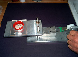
The first question is of both practical and theoretical importance, but for now let’s just say that there are various physical sources of “random” or “unpredictable” data. A user’s mouse movements and typing pattern, (non-solid state) hard drive and network latency, thermal noise, and radioactive decay have all been used as sources for randomness (see discussion in Section 20.8). For example, many Intel chips come with a random number generator built in. One can even build mechanical coin tossing machines (see Figure 20.1).

20.1: A mechanical coin tosser built for Percy Diaconis by Harvard technicians Steve Sansone and Rick Haggerty

In this chapter we focus on the second question: formally modeling probabilistic computation and studying its power. We will show that:

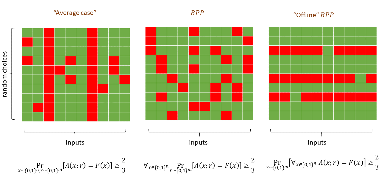
We can define the class \(\mathbf{BPP}\) that captures all Boolean functions that can be computed in polynomial time by a randomized algorithm. Crucially \(\mathbf{BPP}\) is still very much a worst case class of computation: the probability is only over the choice of the random coins of the algorithm, as opposed to the choice of the input.
We can amplify the success probability of randomized algorithms, and as a result the definition of the class \(\mathbf{BPP}\) is equivalent whether or not we require \(2/3\) success, \(0.51\) success or every \(1-2^{-n}\) success.
Though, as is the case for \(\mathbf{P}\) and \(\mathbf{NP}\), there is much we do not know about the class \(\mathbf{BPP}\), we can establish some relations between \(\mathbf{BPP}\) and the other complexity classes we saw before. In particular we will show that \(\mathbf{P} \subseteq \mathbf{BPP} \subseteq \mathbf{EXP}\) and \(\mathbf{BPP} \subseteq \mathbf{P_{/poly}}\).
While the relation between \(\mathbf{BPP}\) and \(\mathbf{NP}\) is not known, we can show that if \(\mathbf{P}=\mathbf{NP}\) then \(\mathbf{BPP}=\mathbf{P}\).
We also show that the concept of \(\mathbf{NP}\) completeness applies equally well if we use randomized algorithms as our model of “efficient computation”. That is, if a single \(\mathbf{NP}\) complete problem has a randomized polynomial-time algorithm, then all of \(\mathbf{NP}\) can be computed in polynomial-time by randomized algorithms.
Finally we will discuss the question of whether \(\mathbf{BPP} = \mathbf{P}\) and show some of the intriguing evidence that the answer might actually be “Yes” using the concept of pseudorandom generators.

Modeling randomized computation

Modeling randomized computation is actually quite easy. We can add the following operations to any programming language such as NAND-TM, NAND-RAM, NAND-CIRC etc..:

foo = RAND()

where foo is a variable. The result of applying this operation is that foo is assigned a random bit in \(\{0,1\}\). (Every time the RAND operation is invoked it returns a fresh independent random bit.) We call the programming languages that are augmented with this extra operation RNAND-TM, RNAND-RAM, and RNAND-CIRC respectively.

Similarly, we can easily define randomized Turing machines as Turing machines in which the transition function \(\delta\) gets as an extra input (in addition to the current state and symbol read from the tape) a bit \(b\) that in each step is chosen at random \(\{0,1\}\). Of course the transition function can ignore this bit (and have the same output regardless of whether \(b=0\) or \(b=1\)), and hence randomized Turing machines generalize deterministic Turing machines.

We can use the RAND() operation to define the notion of a function being computed by a randomized \(T(n)\) time algorithm for every nice time bound \(T:\N \rightarrow \N\), as well as the notion of a finite function being computed by a size \(S\) randomized NAND-CIRC program (or, equivalently, a randomized circuit with \(S\) gates that correspond to either the NAND or coin-tossing operations). However, for simplicity we will not define randomized computation in full generality, but simply focus on the class of functions that are computable by randomized algorithms running in polynomial time, which by historical convention is known as \(\mathbf{BPP}\):

Let \(F: \{0,1\}^*\rightarrow \{0,1\}\). We say that \(F\in \mathbf{BPP}\) if there exist constants \(a,b\in \N\) and an RNAND-TM program \(P\) such that for every \(x\in \{0,1\}^*\), on input \(x\), the program \(P\) halts within at most \(a|x|^b\) steps and

\[ \Pr[ P(x)= F(x)] \geq \tfrac{2}{3} \;\;(20.1) \]

where this probability is taken over the result of the RAND operations of \(P\).

Note that the probability in Equation 20.1 is taken only over the random choices in the execution of \(P\) and not over the choice of the input \(x\). In particular, as discussed in Big Idea 24, \(\mathbf{BPP}\) is still a worst case complexity class, in the sense that if \(F\) is in \(\mathbf{BPP}\) then there is a polynomial-time randomized algorithm that computes \(F\) with probability at least \(2/3\) on every possible (and not just random) input.

The same polynomial-overhead simulation of NAND-RAM programs by NAND-TM programs we saw in Theorem 13.5 extends to randomized programs as well. Hence the class \(\mathbf{BPP}\) is the same regardless of whether it is defined via RNAND-TM or RNAND-RAM programs. Similarly, we could have just as well defined \(\mathbf{BPP}\) using randomized Turing machines.

Because of these equivalences, below we will use the name “polynomial time randomized algorithm” to denote a computation that can be modeled by a polynomial-time RNAND-TM program, RNAND-RAM program, or a randomized Turing machine (or any programming language that includes a coin tossing operation). Since all these models are equivalent up to polynomial factors, you can use your favorite model to capture polynomial-time randomized algorithms without any loss in generality.

Modern programming languages often involve not just the ability to toss a random coin in \(\{0,1\}\) but also to choose an element at random from a set \(S\). Show that you can emulate this primitive using coin tossing. Specifically, show that there is a randomized algorithm \(A\) that, on input a set \(S\) of \(m\) strings of length \(n\), runs in time \(poly(n,m)\) and outputs either an element \(x\in S\) or “fail” such that

Let \(p\) be the probability that \(A\) outputs “fail”, then \(p < 2^{-n}\) (a number small enough that it can be ignored).
For every \(x \in S\), the probability that \(A\) outputs \(x\) is exactly \(\tfrac{1-p}{m}\) (and so the output is uniform over \(S\) if we ignore the tiny probability of failure)

If the size of \(S\) is a power of two, that is \(m=2^\ell\) for some \(\ell\in N\), then we can choose a random element in \(S\) by tossing \(\ell\) coins to obtain a string \(w \in \{0,1\}^\ell\) and then output the \(i\)-th element of \(S\) where \(i\) is the number whose binary representation is \(w\).

If \(S\) is not a power of two, then our first attempt will be to let \(\ell = \ceil{\log m}\) and do the same, but then output the \(i\)-th element of \(S\) if \(i \in [m]\) and output “fail” otherwise. Conditioned on not outputting “fail”, this element is distributed uniformly in \(S\). However, in the worst case, \(2^\ell\) can be almost \(2m\) and so the probability of fail might be close to half. To reduce the failure probability, we can repeat the experiment above \(n\) times. Specifically, we will use the following algorithm

Algorithm 20.2 Sample from set

Input: Set \(S = \{ x_0,\ldots, x_{m-1} \}\) with \(x_i\in \{0,1\}^n\) for all \(i\in [m]\).

Output: Either \(x\in S\) or "fail"

Let \(\ell \leftarrow \lceil \log m \rceil\)

for{\(j = 0,1,\ldots,n-1\)}

Pick \(w \sim \{0,1\}^\ell\)

Let \(i\in [2^\ell]\) be number whose binary representation is \(w\).

if{\(i<m\)}

return \(x_i\)

endif

endfor

return "fail"

Conditioned on not failing, the output of Algorithm 20.2 is uniformly distributed in \(S\). However, since \(2^\ell < 2m\), the probability of failure in each iteration is less than \(1/2\) and so the probability of failure in all of them is at most \((1/2)^{n}= 2^{-n}\).

An alternative view: random coins as an “extra input”

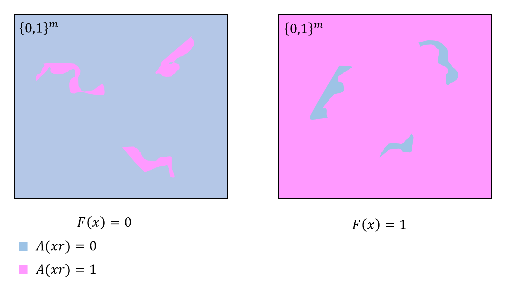
While we presented randomized computation as adding an extra “coin tossing” operation to our programs, we can also model this as being given an additional extra input. That is, we can think of a randomized algorithm \(A\) as a deterministic algorithm \(A'\) that takes two inputs \(x\) and \(r\) where the second input \(r\) is chosen at random from \(\{0,1\}^m\) for some \(m\in \N\) (see Figure 20.2). The equivalence to the Definition 20.1 is shown in the following theorem:

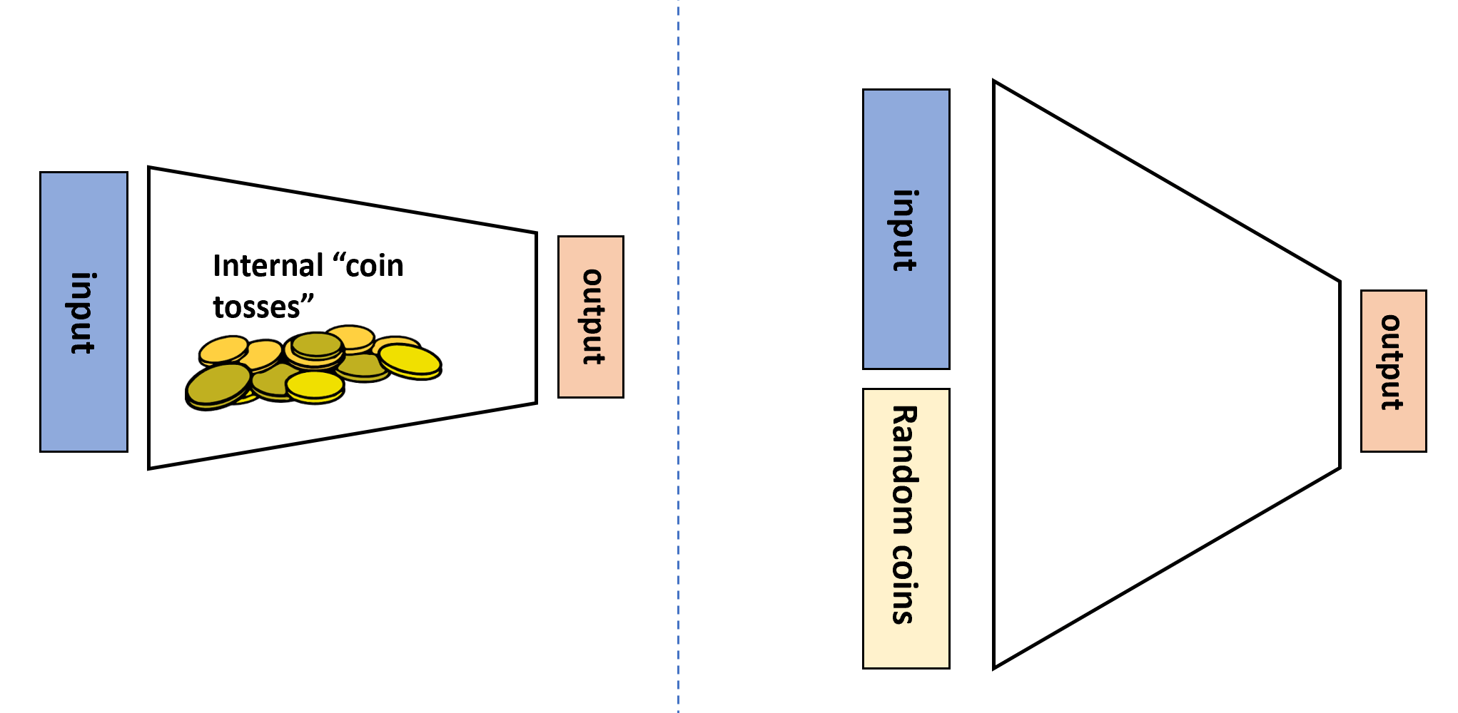
20.2: The two equivalent views of randomized algorithms. We can think of such an algorithm as having access to an internal `RAND()` operation that outputs a random independent value in \(\{0,1\}\) whenever it is invoked, or we can think of it as a deterministic algorithm that in addition to the standard input \(x \in \{0,1\}^n\) obtains an additional auxiliary input \(r \in \{0,1\}^m\) that is chosen uniformly at random.

Let \(F:\{0,1\}^* \rightarrow \{0,1\}\). Then \(F\in \mathbf{BPP}\) if and only if there exists \(a,b\in \N\) and \(G:\{0,1\}^* \rightarrow \{0,1\}\) such that \(G\) is in \(\mathbf{P}\) and for every \(x\in \{0,1\}^*\),

\[ \Pr_{r\sim \{0,1\}^{a|x|^b}} [ G(xr)=F(x)] \geq \tfrac{2}{3} \;\;(20.2)\;. \]

The idea behind the proof is that, as illustrated in Figure 20.2, we can simply replace sampling a random coin with reading a bit from the extra “random input” \(r\) and vice versa. To prove this rigorously we need to work through some slightly cumbersome formal notation. This might be one of those proofs that is easier to work out on your own than to read.

We start by showing the “only if” direction. Let \(F\in \mathbf{BPP}\) and let \(P\) be an RNAND-TM program that computes \(F\) as per Definition 20.1, and let \(a,b\in \N\) be such that on every input of length \(n\), the program \(P\) halts within at most \(an^b\) steps. We will construct a polynomial-time algorithm \(P'\) such that for every \(x\in \{0,1\}^n\), if we set \(m=an^b\), then

\[ \Pr_{r \sim \{0,1\}^{m}}[ P'(xr) = 1] = \Pr[ P(x) = 1 ] \;, \]

where the probability in the right-hand side is taken over the RAND() operations in \(P\). In particular this means that if we define \(G(xr) = P'(xr)\) then the function \(G\) satisfies the conditions of Equation 20.2.

The algorithm \(P'\) will be very simple: it simulates the program \(P\), maintaining a counter \(i\) initialized to \(0\). Every time that \(P\) makes a RAND() operation, the program \(P'\) will supply the result from \(r_i\) and increment \(i\) by one. We will never “run out” of bits, since the running time of \(P\) is at most \(an^b\) and hence it can make at most this number of RAND() calls. The output of \(P'(xr)\) for a random \(r\sim \{0,1\}^m\) will be distributed identically to the output of \(P(x)\).

For the other direction, given a function \(G\in \mathbf{P}\) satisfying the condition Equation 20.2 and a NAND-TM \(P'\) that computes \(G\) in polynomial time, we can construct an RNAND-TM program \(P\) that computes \(F\) in polynomial time. On input \(x\in \{0,1\}^n\), the program \(P\) will simply use the RAND() instruction \(an^b\) times to fill an array R[\(0\)] , \(\ldots\), R[\(an^b-1\)] and then execute the original program \(P'\) on input \(xr\) where \(r_i\) is the \(i\)-th element of the array R. Once again, it is clear that if \(P'\) runs in polynomial time then so will \(P\), and for every input \(x\) and \(r\in \{0,1\}^{an^b}\), the output of \(P\) on input \(x\) and where the coin tosses outcome is \(r\) is equal to \(P'(xr)\).

The characterization of \(\mathbf{BPP}\) in Theorem 20.3 is reminiscent of the characterization of \(\mathbf{NP}\) in Definition 15.1, with the randomness in the case of \(\mathbf{BPP}\) playing the role of the solution in the case of \(\mathbf{NP}\). However, there are important differences between the two:

The definition of \(\mathbf{NP}\) is “one sided”: \(F(x)=1\) if there exists a solution \(w\) such that \(G(xw)=1\) and \(F(x)=0\) if for every string \(w\) of the appropriate length, \(G(xw)=0\). In contrast, the characterization of \(\mathbf{BPP}\) is symmetric with respect to the cases \(F(x)=0\) and \(F(x)=1\).
The relation between \(\mathbf{NP}\) and \(\mathbf{BPP}\) is not immediately clear. It is not known whether \(\mathbf{BPP} \subseteq \mathbf{NP}\), \(\mathbf{NP} \subseteq \mathbf{BPP}\), or these two classes are incomparable. It is however known (with a non-trivial proof) that if \(\mathbf{P}=\mathbf{NP}\) then \(\mathbf{BPP}=\mathbf{P}\) (see Theorem 20.11).
Most importantly, the definition of \(\mathbf{NP}\) is “ineffective,” since it does not yield a way of actually finding whether there exists a solution among the exponentially many possibilities. By contrast, the definition of \(\mathbf{BPP}\) gives us a way to compute the function in practice by simply choosing the second input at random.

“Random tapes”. Theorem 20.3 motivates sometimes considering the randomness of an RNAND-TM (or RNAND-RAM) program as an extra input. As such, if \(A\) is a randomized algorithm that on inputs of length \(n\) makes at most \(m\) coin tosses, we will often use the notation \(A(x;r)\) (where \(x\in \{0,1\}^n\) and \(r\in \{0,1\}^{m}\)) to refer to the result of executing \(x\) when the coin tosses of \(A\) correspond to the coordinates of \(r\). This second, or “auxiliary,” input is sometimes referred to as a “random tape.” This terminology originates from the model of randomized Turing machines.

Success amplification of two-sided error algorithms

The number \(2/3\) might seem arbitrary, but as we’ve seen in Chapter 19 it can be amplified to our liking:

Let \(F:\{0,1\}^* \rightarrow \{0,1\}\) be a Boolean function such that there is a polynomial \(p:\N \rightarrow \N\) and a polynomial-time randomized algorithm \(A\) satisfying that for every \(x\in \{0,1\}^n\),

\[ \Pr[A(x) = F(x)] \geq \frac{1}{2} + \frac{1}{p(n)} \;\;(20.3) \;. \]

Then for every polynomial \(q:\N \rightarrow \N\) there is a polynomial-time randomized algorithm \(B\) satisfying for every \(x\in \{0,1\}^n\),

\[ \Pr[B(x) = F(x)] \geq 1 - 2^{-q(n)} \;. \]

We can amplify the success of randomized algorithms to a value that is arbitrarily close to \(1\).

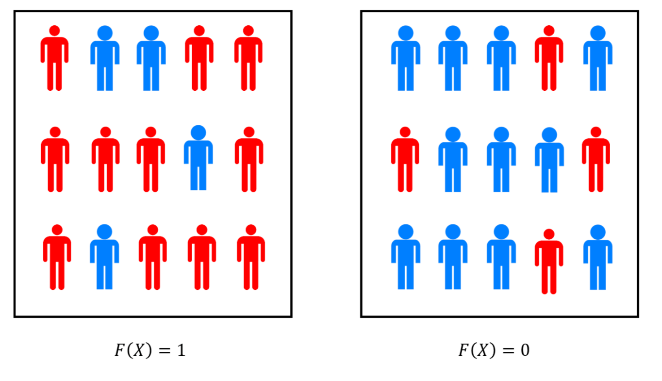
The proof is the same as we’ve seen before in the case of maximum cut and other examples. We use the Chernoff bound to argue that if \(A\) computes \(F\) with probability at least \(\tfrac{1}{2} + \epsilon\) and we run it \(O(k/\epsilon^2)\) times, each time using fresh and independent random coins, then the probability that the majority of the answers will not be correct will be less than \(2^{-k}\). Amplification can be thought of as a “polling” of the choices for randomness for the algorithm (see Figure 20.3).

Let \(A\) be an algorithm satisfying Equation 20.3. Set \(\epsilon = \tfrac{1}{p(n)}\) and \(k = q(n)\) where \(p,q\) are the polynomials in the theorem statement. We can run \(P\) on input \(x\) for \(t=10k/\epsilon^2\) times, using fresh randomness in each execution, and compute the outputs \(y_0,\ldots,y_{t-1}\). We output the value \(y\) that appeared the largest number of times. Let \(X_i\) be the random variable that is equal to \(1\) if \(y_i = F(x)\) and equal to \(0\) otherwise. The random variables \(X_0,\ldots,X_{t-1}\) are i.i.d. and satisfy \(\E [X_i] = \Pr[ X_i = 1] \geq 1/2 + \epsilon\), and hence by linearity of expectation \(\mathbb{E}[\sum_{i=0}^{t-1} X_i] \geq t(1/2 + \epsilon)\). For the plurality value to be incorrect, it must hold that \(\sum_{i=0}^{t-1} X_i \leq t/2\), which means that \(\sum_{i=0}^{t-1}X_i\) is at least \(\epsilon t\) far from its expectation. Hence by the Chernoff bound (Theorem 18.12), the probability that the plurality value is not correct is at most \(2e^{-\epsilon^2 t}\), which is smaller than \(2^{-k}\) for our choice of \(t\).

20.3: If \(F\in\mathbf{BPP}\) then there is a randomized polynomial-time algorithm \(P\) with the following property: In the case \(F(x)=0\) two thirds of the “population” of random choices satisfy \(P(x;r)=0\) and in the case \(F(x)=1\) two thirds of the population satisfy \(P(x;r)=1\). We can think of amplification as a form of “polling” of the choices of randomness. By the Chernoff bound, if we poll a sample of \(O(\tfrac{\log(1/\delta)}{\epsilon^2})\) random choices \(r\), then with probability at least \(1-\delta\), the fraction of \(r\)’s in the sample satisfying \(P(x;r)=1\) will give us an estimate of the fraction of the population within an \(\epsilon\) margin of error. This is the same calculation used by pollsters to determine the needed sample size in their polls.

\(\mathbf{BPP}\) and \(\mathbf{NP}\) completeness

Since “noisy processes” abound in nature, randomized algorithms can be realized physically, and so it is reasonable to propose \(\mathbf{BPP}\) rather than \(\mathbf{P}\) as our mathematical model for “feasible” or “tractable” computation. One might wonder if this makes all the previous chapters irrelevant, and in particular if the theory of \(\mathbf{NP}\) completeness still applies to probabilistic algorithms. Fortunately, the answer is Yes:

Suppose that \(F\) is \(\mathbf{NP}\)-hard and \(F\in \mathbf{BPP}\). Then \(\mathbf{NP} \subseteq \mathbf{BPP}\).

Before seeing the proof, note that Theorem 20.6 implies that if there was a randomized polynomial time algorithm for any \(\mathbf{NP}\)-complete problem such as \(3\ensuremath{\mathit{SAT}}\), \(\ensuremath{\mathit{ISET}}\) etc., then there would be such an algorithm for every problem in \(\mathbf{NP}\). Thus, regardless of whether our model of computation is deterministic or randomized algorithms, \(\mathbf{NP}\) complete problems retain their status as the “hardest problems in \(\mathbf{NP}\).”

The idea is to simply run the reduction as usual, and plug it into the randomized algorithm instead of a deterministic one. It would be an excellent exercise, and a way to reinforce the definitions of \(\mathbf{NP}\)-hardness and randomized algorithms, for you to work out the proof for yourself. However for the sake of completeness, we include this proof below.

Suppose that \(F\) is \(\mathbf{NP}\)-hard and \(F\in \mathbf{BPP}\). We will now show that this implies that \(\mathbf{NP} \subseteq \mathbf{BPP}\). Let \(G \in \mathbf{NP}\). By the definition of \(\mathbf{NP}\)-hardness, it follows that \(G \leq_p F\), or that in other words there exists a polynomial-time computable function \(R:\{0,1\}^* \rightarrow \{0,1\}^*\) such that \(G(x)=F(R(x))\) for every \(x\in \{0,1\}^*\). Now if \(F\) is in \(\mathbf{BPP}\) then there is a polynomial-time RNAND-TM program \(P\) such that

\[ \Pr[ P(y)= F(y) ] \geq 2/3 \;\;(20.4) \]

for every \(y\in \{0,1\}^*\) (where the probability is taken over the random coin tosses of \(P\)). Hence we can get a polynomial-time RNAND-TM program \(P'\) to compute \(G\) by setting \(P'(x)=P(R(x))\). By Equation 20.4 \(\Pr[ P'(x) = F(R(x))] \geq 2/3\) and since \(F(R(x))=G(x)\) this implies that \(\Pr[ P'(x) = G(x)] \geq 2/3\), which proves that \(G \in \mathbf{BPP}\).

Most of the results we’ve seen about \(\mathbf{NP}\) hardness, including the search to decision reduction of Theorem 16.1, the decision to optimization reduction of Theorem 16.3, and the quantifier elimination result of Theorem 16.6, all carry over in the same way if we replace \(\mathbf{P}\) with \(\mathbf{BPP}\) as our model of efficient computation. Thus if \(\mathbf{NP} \subseteq \mathbf{BPP}\) then we get essentially all of the strange and wonderful consequences of \(\mathbf{P}=\mathbf{NP}\). Unsurprisingly, we cannot rule out this possibility. In fact, unlike \(\mathbf{P}=\mathbf{EXP}\), which is ruled out by the time hierarchy theorem, we don’t even know how to rule out the possibility that \(\mathbf{BPP}=\mathbf{EXP}\)! Thus a priori it’s possible (though seems highly unlikely) that randomness is a magical tool that allows us to speed up arbitrary exponential time computation.¹ Nevertheless, as we discuss below, it is believed that randomization’s power is much weaker and \(\mathbf{BPP}\) lies in much more “pedestrian” territory.

The power of randomization

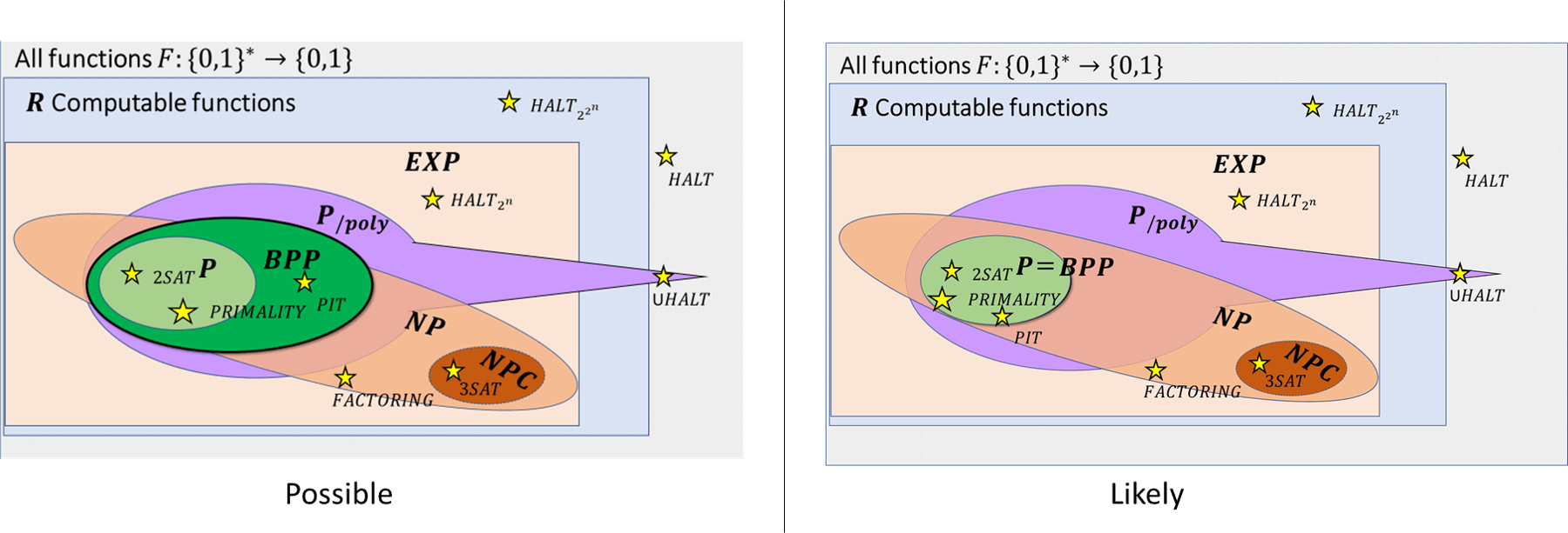
A major question is whether randomization can add power to computation. Mathematically, we can phrase this as the following question: does \(\mathbf{BPP}=\mathbf{P}\)? Given what we’ve seen so far about the relations of other complexity classes such as \(\mathbf{P}\) and \(\mathbf{NP}\), or \(\mathbf{NP}\) and \(\mathbf{EXP}\), one might guess that:

We do not know the answer to this question.
But we suspect that \(\mathbf{BPP}\) is different than \(\mathbf{P}\).

One would be correct about the former, but wrong about the latter. As we will see, we do in fact have reasons to believe that \(\mathbf{BPP}=\mathbf{P}\). This can be thought of as supporting the extended Church Turing hypothesis that deterministic polynomial-time Turing machines capture what can be feasibly computed in the physical world.

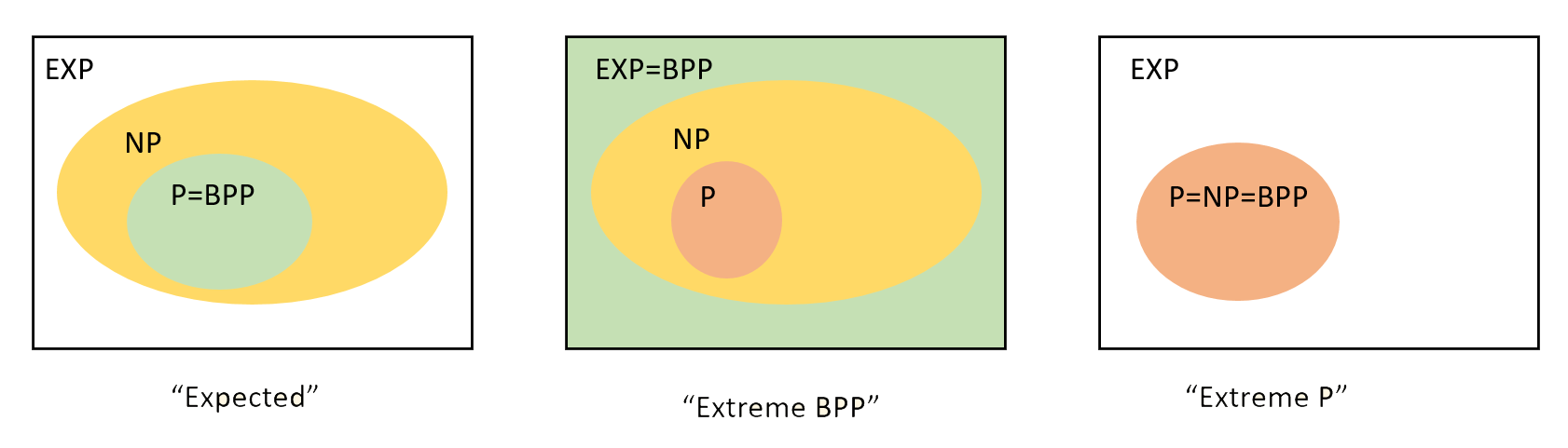
We now survey some of the relations that are known between \(\mathbf{BPP}\) and other complexity classes we have encountered. (See also Figure 20.4.)

20.4: Some possibilities for the relations between \(\mathbf{BPP}\) and other complexity classes. Most researchers believe that \(\mathbf{BPP}=\mathbf{P}\) and that these classes are *not* powerful enough to solve \(\mathbf{NP}\)-complete problems, let alone all problems in \(\mathbf{EXP}\). However, we have not even been able yet to rule out the possibility that randomness is a “silver bullet” that allows exponential speedup on all problems, and hence \(\mathbf{BPP}=\mathbf{EXP}\). As we’ve already seen, we also can’t rule out that \(\mathbf{P}=\mathbf{NP}\). Interestingly, in the latter case, \(\mathbf{P}=\mathbf{BPP}\).

Solving \(\mathbf{BPP}\) in exponential time

It is not hard to see that if \(F\) is in \(\mathbf{BPP}\) then it can be computed in exponential time.

\(\mathbf{BPP} \subseteq \mathbf{EXP}\)

The proof of Theorem 20.7 readily follows by enumerating over all the (exponentially many) choices for the random coins. We omit the formal proof, as doing it by yourself is an excellent way to get comfortable with Definition 20.1.

Simulating randomized algorithms by circuits

We have seen in Theorem 13.12 that if \(F\) is in \(\mathbf{P}\), then there is a polynomial \(p:\N \rightarrow \N\) such that for every \(n\), the restriction \(F_{\upharpoonright n}\) of \(F\) to inputs \(\{0,1\}^n\) is in \(\ensuremath{\mathit{SIZE}}(p(n))\). (In other words, that \(\mathbf{P} \subseteq \mathbf{P_{/poly}}\).) A priori it is not at all clear that the same holds for a function in \(\mathbf{BPP}\), but this does turn out to be the case.

20.5: The possible guarantees for a randomized algorithm \(A\) computing some function \(F\). In the tables above, the columns correspond to different inputs and the rows to different choices of the random tape. A cell at position \(r,x\) is colored green if \(A(x;r)=F(x)\) (i.e., the algorithm outputs the correct answer) and red otherwise. The standard \(\mathbf{BPP}\) guarantee corresponds to the middle figure, where for every input \(x\), at least two thirds of the choices \(r\) for a random tape will result in \(A\) computing the correct value. That is, every column is colored green in at least two thirds of its coordinates. In the left figure we have an “average case” guarantee where the algorithm is only guaranteed to output the correct answer with probability two thirds over a *random* input (i.e., at most one third of the total entries of the table are colored red, but there could be an all red column). The right figure corresponds to the “offline \(\mathbf{BPP}\)” case, with probability at least two thirds over the random choice \(r\), \(r\) will be good for *every* input. That is, at least two thirds of the rows are all green. Theorem 20.8 (\(\mathbf{BPP} \subseteq \mathbf{P_{/poly}}\)) is proven by amplifying the success of a \(\mathbf{BPP}\) algorithm until we have the “offline \(\mathbf{BPP}\)” guarantee, and then hardwiring the choice of the randomness \(r\) to obtain a non-uniform deterministic algorithm.

\(\mathbf{BPP} \subseteq \mathbf{P_{/poly}}\).

That is, for every \(F\in \mathbf{BPP}\), there exist some \(a,b\in \N\) such that for every \(n>0\), \(F_{\upharpoonright n} \in \ensuremath{\mathit{SIZE}}(an^b)\) where \(F_{\upharpoonright n}\) is the restriction of \(F\) to inputs in \(\{0,1\}^n\).

The idea behind the proof is that we can first amplify by repetition the probability of success from \(2/3\) to \(1-0.1 \cdot 2^{-n}\). This will allow us to show that for every \(n\in\N\) there exists a single fixed choice of “favorable coins” which is a string \(r\) of length polynomial in \(n\) such that if \(r\) is used for the randomness then we output the right answer on all of the possible \(2^n\) inputs. We can then use the standard “unravelling the loop” technique to transform an RNAND-TM program to an RNAND-CIRC program, and “hardwire” the favorable choice of random coins to transform the RNAND-CIRC program into a plain old deterministic NAND-CIRC program.

Suppose that \(F\in \mathbf{BPP}\). Let \(P\) be a polynomial-time RNAND-TM program that computes \(F\) as per Definition 20.1. Using Theorem 20.5, we can amplify the success probability of \(P\) to obtain an RNAND-TM program \(P'\) that is at most a factor of \(O(n)\) slower (and hence still polynomial time) such that for every \(x\in \{0,1\}^n\)

\[ \Pr_{r \sim \{0,1\}^m}[ P'(x;r)=F(x)] \geq 1 - 0.1\cdot 2^{-n} \;, \;\;(20.5) \]

where \(m\) is the number of coin tosses that \(P'\) uses on inputs of length \(n\). We use the notation \(P'(x;r)\) to denote the execution of \(P'\) on input \(x\) and when the result of the coin tosses corresponds to the string \(r\).

For every \(x\in \{0,1\}^n\), define the “bad” event \(B_x\) to hold if \(P'(x) \neq F(x)\), where the sample space for this event consists of the coins of \(P'\). Then by Equation 20.5, \(\Pr[B_x] \leq 0.1\cdot 2^{-n}\) for every \(x \in \{0,1\}^n\). Since there are \(2^n\) many such \(x\)’s, by the union bound we see that the probability that the union of the events \(\{ B_x \}_{x\in \{0,1\}^n}\) is at most \(0.1\). This means that if we choose \(r \sim \{0,1\}^m\), then with probability at least \(0.9\) it will be the case that for every \(x\in \{0,1\}^n\), \(F(x)=P'(x;r)\). (Indeed, otherwise the event \(B_x\) would hold for some \(x\).) In particular, because of the mere fact that the probability of \(\cup_{x \in \{0,1\}^n} B_x\) is smaller than \(1\), this means that there exists a particular \(r^* \in \{0,1\}^m\) such that

\[P'(x;r^*)=F(x) \;\;(20.6) \]

for every \(x\in \{0,1\}^n\).

Now let us use the standard “unravelling the loop” technique and transform \(P'\) into a NAND-CIRC program \(Q\) of polynomial in \(n\) size, such that \(Q(xr)=P'(x;r)\) for every \(x\in \{0,1\}^n\) and \(r \in \{0,1\}^m\). Then by “hardwiring” the values \(r^*_0,\ldots,r^*_{m-1}\) in place of the last \(m\) inputs of \(Q\), we obtain a new NAND-CIRC program \(Q_{r^*}\) that satisfies by Equation 20.6 that \(Q_{r^*}(x)=F(x)\) for every \(x\in \{0,1\}^n\). This demonstrates that \(F_{\upharpoonright n}\) has a polynomial-sized NAND-CIRC program, hence completing the proof of Theorem 20.8.

Derandomization

The proof of Theorem 20.8 can be summarized as follows: we can replace a \(poly(n)\)-time algorithm that tosses coins as it runs with an algorithm that uses a single set of coin tosses \(r^* \in \{0,1\}^{poly(n)}\) which will be good enough for all inputs of size \(n\). Another way to say it is that for the purposes of computing functions, we do not need “online” access to random coins and can generate a set of coins “offline” ahead of time, before we see the actual input.

But this does not really help us with answering the question of whether \(\mathbf{BPP}\) equals \(\mathbf{P}\), since we still need to find a way to generate these “offline” coins in the first place. To derandomize an RNAND-TM program we will need to come up with a single deterministic algorithm that will work for all input lengths. That is, unlike in the case of RNAND-CIRC programs, we cannot choose for every input length \(n\) some string \(r^* \in \{0,1\}^{poly(n)}\) to use as our random coins.

Can we derandomize randomized algorithms, or does randomness add an inherent extra power for computation? This is a fundamentally interesting question but is also of practical significance. Ever since people started to use randomized algorithms during the Manhattan project, they have been trying to remove the need for randomness and replace it with numbers that are selected through some deterministic process. Throughout the years this approach has often been used successfully, though there have been a number of failures as well.²

A common approach people used over the years was to replace the random coins of the algorithm by a “randomish looking” string that they generated through some arithmetic progress. For example, one can use the digits of \(\pi\) for the random tape. Using these type of methods corresponds to what von Neumann referred to as a “state of sin”. (Though this is a sin that he himself frequently committed, as generating true randomness in sufficient quantity was and still is often too expensive.) The reason that this is considered a “sin” is that such a procedure will not work in general. For example, it is easy to modify any probabilistic algorithm \(A\) such as the ones we have seen in Chapter 19, to an algorithm \(A'\) that is guaranteed to fail if the random tape happens to equal the digits of \(\pi\). This means that the procedure “replace the random tape by the digits of \(\pi\)” does not yield a general way to transform a probabilistic algorithm to a deterministic one that will solve the same problem. Of course, this procedure does not always fail, but we have no good way to determine when it fails and when it succeeds. This reasoning is not specific to \(\pi\) and holds for every deterministically produced string, whether it obtained by \(\pi\), \(e\), the Fibonacci series, or anything else.

An algorithm that checks if its random tape is equal to \(\pi\) and then fails seems to be quite silly, but this is but the “tip of the iceberg” for a very serious issue. Time and again people have learned the hard way that one needs to be very careful about producing random bits using deterministic means. As we will see when we discuss cryptography, many spectacular security failures and break-ins were the result of using “insufficiently random” coins.

Pseudorandom generators

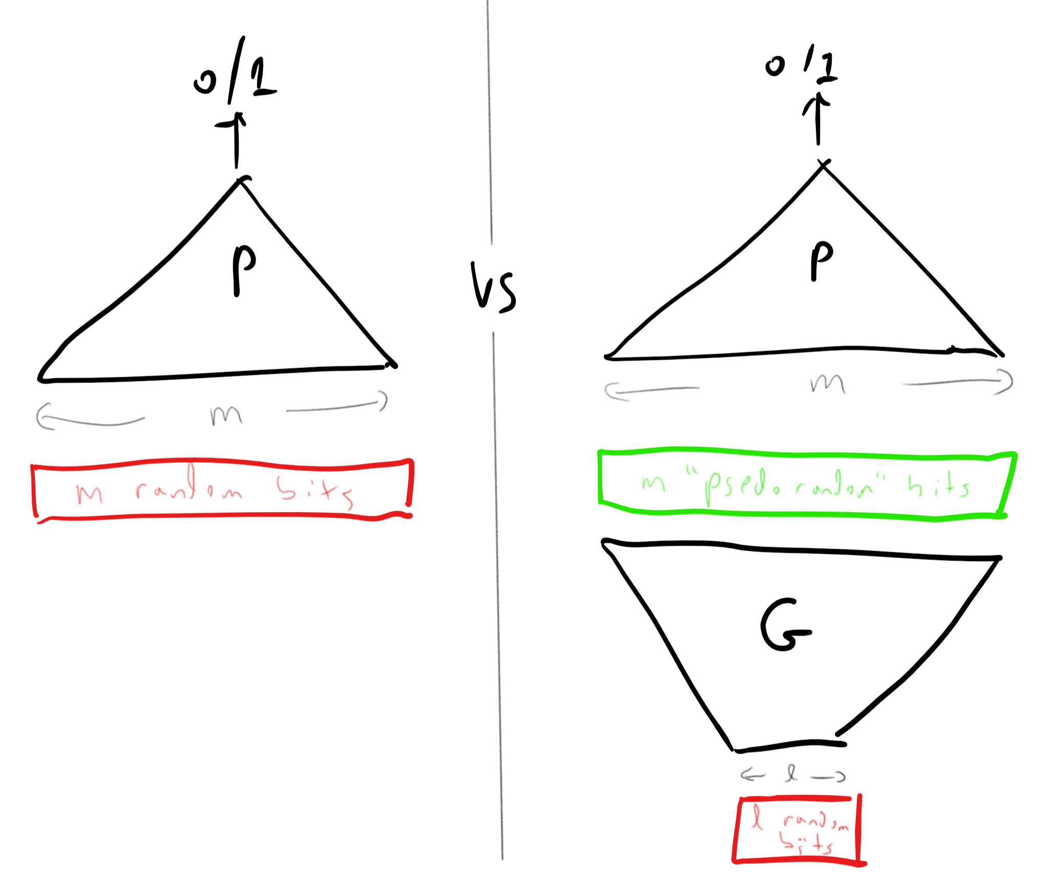
So, we can’t use any single string to “derandomize” a probabilistic algorithm. It turns out however, that we can use a collection of strings to do so. Another way to think about it is that rather than trying to eliminate the need for randomness, we start by focusing on reducing the amount of randomness needed. (Though we will see that if we reduce the randomness sufficiently, we can eventually get rid of it altogether.)

We make the following definition:

A function \(G:\{0,1\}^\ell \rightarrow \{0,1\}^m\) is a \((T,\epsilon)\)-pseudorandom generator if for every circuit \(C\) with \(m\) inputs, one output, and at most \(T\) gates,

\[ \left| \Pr_{s\sim \{0,1\}^\ell}[C(G(s))=1] - \Pr_{r \sim \{0,1\}^m}[C(r)=1] \right| < \epsilon \;\;(20.7) \]

20.6: A pseudorandom generator \(G\) maps a short string \(s\in \{0,1\}^\ell\) into a long string \(r\in \{0,1\}^m\) such that a small program/circuit \(P\) cannot distinguish between the case that it is provided a random input \(r \sim \{0,1\}^m\) and the case that it is provided a “pseudorandom” input of the form \(r=G(s)\) where \(s \sim \{0,1\}^\ell\). The short string \(s\) is sometimes called the *seed* of the pseudorandom generator, as it is a small object that can be thought as yielding a large “tree of randomness”.

This is a definition that’s worth reading more than once, and spending some time to digest it. Note that it takes several parameters:

\(T\) is the limit on the number of gates of the circuit \(C\) that the generator needs to “fool”. The larger \(T\) is, the stronger the generator.
\(\epsilon\) is how close the output of the pseudorandom generator is to the true uniform distribution over \(\{0,1\}^m\). The smaller \(\epsilon\) is, the stronger the generator.
\(\ell\) is the input length and \(m\) is the output length. If \(\ell \geq m\) then it is trivial to come up with such a generator: on input \(s\in \{0,1\}^\ell\), we can output \(s_0,\ldots,s_{m-1}\). In this case \(\Pr_{s\sim \{0,1\}^\ell}[ P(G(s))=1]\) will simply equal \(\Pr_{r\sim \{0,1\}^m}[ P(r)=1]\), no matter how many lines \(P\) has. So, the smaller \(\ell\) is and the larger \(m\) is, the stronger the generator, and to get anything non-trivial, we need \(m>\ell\).

Furthermore note that although our eventual goal is to fool probabilistic randomized algorithms that take an unbounded number of inputs, Definition 20.9 refers to finite and deterministic NAND-CIRC programs.

We can think of a pseudorandom generator as a “randomness amplifier.” It takes an input \(s\) of \(\ell\) bits chosen at random and expands these \(\ell\) bits into an output \(r\) of \(m>\ell\) pseudorandom bits. If \(\epsilon\) is small enough then the pseudorandom bits will “look random” to any NAND-CIRC program that is not too big. Still, there are two questions we haven’t answered:

What reason do we have to believe that pseudorandom generators with non-trivial parameters exist?
Even if they do exist, why would such generators be useful to derandomize randomized algorithms? After all, Definition 20.9 does not involve RNAND-TM or RNAND-RAM programs, but rather deterministic NAND-CIRC programs with no randomness and no loops.

We will now (partially) answer both questions. For the first question, let us come clean and confess we do not know how to prove that interesting pseudorandom generators exist. By interesting we mean pseudorandom generators that satisfy that \(\epsilon\) is some small constant (say \(\epsilon<1/3\)), \(m>\ell\), and the function \(G\) itself can be computed in \(poly(m)\) time. Nevertheless, Lemma 20.12 (whose statement and proof is deferred to the end of this chapter) shows that if we only drop the last condition (polynomial-time computability), then there do in fact exist pseudorandom generators where \(m\) is exponentially larger than \(\ell\).

At this point you might want to skip ahead and look at the statement of Lemma 20.12. However, since its proof is somewhat subtle, I recommend you defer reading it until you’ve finished reading the rest of this chapter.

From existence to constructivity

The fact that there exists a pseudorandom generator does not mean that there is one that can be efficiently computed. However, it turns out that we can turn complexity “on its head” and use the assumed non-existence of fast algorithms for problems such as 3SAT to obtain pseudorandom generators that can then be used to transform randomized algorithms into deterministic ones. This is known as the Hardness vs Randomness paradigm. A number of results along those lines, most of which are outside the scope of this course, have led researchers to believe the following conjecture:

Optimal PRG conjecture: There is a polynomial-time computable function \(\ensuremath{\mathit{PRG}}:\{0,1\}^* \rightarrow \{0,1\}\) that yields an exponentially secure pseudorandom generator.

Specifically, there exists a constant \(\delta >0\) such that for every \(\ell\) and \(m < 2^{\delta \ell}\), if we define \(G:\{0,1\}^\ell \rightarrow \{0,1\}^m\) as \(G(s)_i = \ensuremath{\mathit{PRG}}(s,i)\) for every \(s\in \{0,1\}^\ell\) and \(i \in [m]\), then \(G\) is a \((2^{\delta \ell},2^{-\delta \ell})\) pseudorandom generator.

The “optimal PRG conjecture” is worth while reading more than once. What it posits is that we can obtain a \((T,\epsilon)\) pseudorandom generator \(G\) such that every output bit of \(G\) can be computed in time polynomial in the length \(\ell\) of the input, where \(T\) is exponentially large in \(\ell\) and \(\epsilon\) is exponentially small in \(\ell\). (Note that we could not hope for the entire output to be computable in \(\ell\), as just writing the output down will take too long.)

To understand why we call such a pseudorandom generator “optimal,” it is a great exercise to convince yourself that, for example, there does not exist a \((2^{1.1\ell},2^{-1.1\ell})\) pseudorandom generator (in fact, the number \(\delta\) in the conjecture must be smaller than \(1\)). To see that we can’t have \(T \gg 2^{\ell}\), note that if we allow a NAND-CIRC program with much more than \(2^\ell\) lines then this NAND-CIRC program could “hardwire” inside it all the outputs of \(G\) on all its \(2^\ell\) inputs, and use that to distinguish between a string of the form \(G(s)\) and a uniformly chosen string in \(\{0,1\}^m\). To see that we can’t have \(\epsilon \ll 2^{-\ell}\), note that by guessing the input \(s\) (which will be successful with probability \(2^{-\ell}\)), we can obtain a small (i.e., \(O(\ell)\) line) NAND-CIRC program that achieves a \(2^{-\ell}\) advantage in distinguishing a pseudorandom and uniform input. Working out these details is a highly recommended exercise.

We emphasize again that the optimal PRG conjecture is, as its name implies, a conjecture, and we still do not know how to prove it. In particular, it is stronger than the conjecture that \(\mathbf{P} \neq \mathbf{NP}\). But we do have some evidence for its truth. There is a spectrum of different types of pseudorandom generators, and there are weaker assumptions than the optimal PRG conjecture that suffice to prove that \(\mathbf{BPP}=\mathbf{P}\). In particular this is known to hold under the assumption that there exists a function \(F\in \mathbf{TIME}(2^{O(n)})\) and \(\epsilon >0\) such that for every sufficiently large \(n\), \(F_{\upharpoonright n}\) is not in \(\ensuremath{\mathit{SIZE}}(2^{\epsilon n})\). The name “Optimal PRG conjecture” is non-standard. This conjecture is sometimes known in the literature as the existence of exponentially strong pseudorandom functions.³

Usefulness of pseudorandom generators

We now show that optimal pseudorandom generators are indeed very useful, by proving the following theorem:

Suppose that the optimal PRG conjecture is true. Then \(\mathbf{BPP}=\mathbf{P}\).

The optimal PRG conjecture tells us that we can achieve exponential expansion of \(\ell\) truly random coins into as many as \(2^{\delta \ell}\) “pseudorandom coins.” Looked at from the other direction, it allows us to reduce the need for randomness by taking an algorithm that uses \(m\) coins and converting it into an algorithm that only uses \(O(\log m)\) coins. Now an algorithm of the latter type by can be made fully deterministic by enumerating over all the \(2^{O(\log m)}\) (which is polynomial in \(m\)) possibilities for its random choices.

We now proceed with the proof details.

Let \(F\in \mathbf{BPP}\) and let \(P\) be a NAND-TM program and \(a,b,c,d\) constants such that for every \(x\in \{0,1\}^n\), \(P(x)\) runs in at most \(c \cdot n^d\) steps and \(\Pr_{r\sim \{0,1\}^m}[ P(x;r) = F(x) ] \geq 2/3\). By “unrolling the loop” and hardwiring the input \(x\), we can obtain for every input \(x\in \{0,1\}^n\) a NAND-CIRC program \(Q_x\) of at most, say, \(T=10c \cdot n^d\) lines, that takes \(m\) bits of input and such that \(Q(r)=P(x;r)\).

Now suppose that \(G:\{0,1\}^\ell \rightarrow \{0,1\}\) is a \((T,0.1)\) pseudorandom generator. Then we could deterministically estimate the probability \(p(x)= \Pr_{r\sim \{0,1\}^m}[ Q_x(r) = 1 ]\) up to \(0.1\) accuracy in time \(O(T \cdot 2^\ell \cdot m \cdot cost(G))\) where \(cost(G)\) is the time that it takes to compute a single output bit of \(G\).

The reason is that we know that \(\tilde{p}(x)= \Pr_{s \sim \{0,1\}^\ell}[ Q_x(G(s)) = 1]\) will give us such an estimate for \(p(x)\), and we can compute the probability \(\tilde{p}(x)\) by simply trying all \(2^\ell\) possibillites for \(s\). Now, under the optimal PRG conjecture we can set \(T = 2^{\delta \ell}\) or equivalently \(\ell = \tfrac{1}{\delta}\log T\), and our total computation time is polynomial in \(2^\ell = T^{1/\delta}\). Since \(T \leq 10c \cdot n^d\), this running time will be polynomial in \(n\).

This completes the proof, since we are guaranteed that \(\Pr_{r\sim \{0,1\}^m}[ Q_x(r) = F(x) ] \geq 2/3\), and hence estimating the probability \(p(x)\) to within \(0.1\) accuracy is sufficient to compute \(F(x)\).

\(\mathbf{P}=\mathbf{NP}\) and \(\mathbf{BPP}\) vs \(\mathbf{P}\)

Two computational complexity questions that we cannot settle are:

Is \(\mathbf{P}=\mathbf{NP}\)? Where we believe the answer is negative.
Is \(\mathbf{BPP}=\mathbf{P}\)? Where we believe the answer is positive.

However we can say that the “conventional wisdom” is correct on at least one of these questions. Namely, if we’re wrong on the first count, then we’ll be right on the second one:

If \(\mathbf{P}=\mathbf{NP}\) then \(\mathbf{BPP}=\mathbf{P}\).

Before reading the proof, it is instructive to think why this result is not “obvious.” If \(\mathbf{P}=\mathbf{NP}\) then given any randomized algorithm \(A\) and input \(x\), we will be able to figure out in polynomial time if there is a string \(r\in \{0,1\}^m\) of random coins for \(A\) such that \(A(xr)=1\). The problem is that even if \(\Pr_{r\sim \{0,1\}^m}[A(xr)=F(x)] \geq 0.9999\), it can still be the case that even when \(F(x)=0\) there exists a string \(r\) such that \(A(xr)=1\).

The proof is rather subtle. It is much more important that you understand the statement of the theorem than that you follow all the details of the proof.

The construction follows the “quantifier elimination” idea which we have seen in Theorem 16.6. We will show that for every \(F \in \mathbf{BPP}\), we can reduce the question of some input \(x\) satisfies \(F(x)=1\) to the question of whether a formula of the form \(\exists_{u\in \{0,1\}^m} \forall_{v \in \{0,1\}^k} P(u,v)\) is true, where \(m,k\) are polynomial in the length of \(x\) and \(P\) is polynomial-time computable. By Theorem 16.6, if \(\mathbf{P}=\mathbf{NP}\) then we can decide in polynomial time whether such a formula is true or false.

The idea behind this construction is that using amplification we can obtain a randomized algorithm \(A\) for computing \(F\) using \(m\) coins such that for every \(x\in \{0,1\}^n\), if \(F(x)=0\) then the set \(S \subseteq \{0,1\}^m\) of coins that make \(A\) output \(1\) is extremely tiny (i.e., exponentially small relative to \(2^m\)), and if \(F(x)=1\) then \(S\) is very large (of size close to \(2^m\)). We then consider “shifts” of the set \(S\): sets of the form \(S \oplus s\) where \(s\in \{0,1\}^m\) is some string, where \(S \oplus s\) is defined as \(\{ r \oplus s \;|\; r \in S \}\). Note that for every such shift \(s\), the cardinality of \(S \oplus s\) is the same as the cardinality of \(S\). Hence, if \(F(x)=0\), and so \(S\) is “tiny”, then for every polynomial number of shifts \(s_0,\ldots,s_k \in \{0,1\}^m\), the union of the sets \(S \oplus s_i\) will not cover \(\{0,1\}^m\). On the other hand, we will show that if \(S\) is very large, then there exists a polynomial number of such shifts such as \(\cup_{i=0}^{k-1} (S \oplus s_i) = \{0,1\}^m\).

We can express the condition that there exists \(s_0,\ldots,s_{k-1}\) such that \(\cup_{i\in [k]} (S \oplus s_i) = \{0,1\}^m\) as a statement with a constant number of quantifiers. (Specifically, this condition holds if for every \(y\in \{0,1\}^m\), there exists \(s \in S\) and \(i\in \{0,\ldots,k-1\}\) such that \(y=s\oplus s_i\).)

20.7: If \(F\in \mathbf{BPP}\) then through amplification we can ensure that there is an algorithm \(A\) to compute \(F\) on \(n\)-length inputs and using \(m\) coins such that \(\Pr_{r\sim \{0,1\}^m}[ A(xr)\neq F(x)] \ll 1/poly(m)\). Hence if \(F(x)=1\) then almost all of the \(2^m\) choices for \(r\) will cause \(A(xr)\) to output \(1\), while if \(F(x)=0\) then \(A(xr)=0\) for almost all \(r\)’s. To prove the Sipser–Gács Theorem we consider several “shifts” of the set \(S \subseteq \{0,1\}^m\) of the coins \(r\) such that \(A(xr)=1\). If \(F(x)=1\) then we can find a set of \(k\) shifts \(s_0,\ldots,s_{k-1}\) for which \(\cup_{i\in [k]} (S \oplus s_i) = \{0,1\}^m\). If \(F(x)=0\) then for every such set \(|\cup_{i\in [k]} S_i| \leq k |S| \ll 2^m\). We can phrase the question of whether there is such a set of shifts using a constant number of quantifiers, and so can solve it in polynomial time if \(\mathbf{P}=\mathbf{NP}\).

Let \(F \in \mathbf{BPP}\). Using Theorem 20.5, there exists a polynomial-time algorithm \(A\) such that for every \(x\in \{0,1\}^n\), \(\Pr_{r \in \{0,1\}^m}[ A(xr)=F(x)] \geq 1 - 2^{-n}\) where \(m\) is polynomial in \(n\). In particular (since an exponential dominates a polynomial, and we can always assume \(n\) is sufficiently large), it holds that

\[ \Pr_{r \in \{0,1\}^m}[ A(xr)=F(x)] \geq 1 - \tfrac{1}{10m^2} \;. \;\;(20.8) \]

Let \(x\in \{0,1\}^n\), and let \(S_x \subseteq \{0,1\}^m\) be the set \(\{ r\in \{0,1\}^m \;:\; A(xr)=1 \}\). By our assumption, if \(F(x)=0\) then \(|S_x| \leq \tfrac{1}{10m^2}2^{m}\) and if \(F(x)=1\) then \(|S_x| \geq (1-\tfrac{1}{10m^2})2^m\).

For a set \(S \subseteq \{0,1\}^m\) and a string \(s\in \{0,1\}^m\), we define the set \(S \oplus s\) to be \(\{ r \oplus s \;:\; r\in S \}\) where \(\oplus\) denotes the XOR operation. That is, \(S \oplus s\) is the set \(S\) “shifted” by \(s\). Note that \(|S \oplus s| = |S|\). (Please make sure that you see why this is true.)

The heart of the proof is the following two claims:

CLAIM I: For every subset \(S \subseteq \{0,1\}^m\), if \(|S| \leq \tfrac{1}{1000m}2^m\), then for every \(s_0,\ldots,s_{100m-1} \in \{0,1\}^m\), \(\cup_{i\in [100m]} (S \oplus s_i) \subsetneq \{0,1\}^m\).

CLAIM II: For every subset \(S \subseteq \{0,1\}^m\), if \(|S| \geq \tfrac{1}{2}2^m\) then there exist a set of string \(s_0,\ldots,s_{100m-1}\) such that \(\cup_{i\in [100m]} (S \oplus s_i) = \{0,1\}^m\).

CLAIM I and CLAIM II together imply the theorem. Indeed, they mean that under our assumptions, for every \(x\in \{0,1\}^n\), \(F(x)=1\) if and only if

\[ \exists_{s_0,\ldots, s_{100m-1} \in \{0,1\}^m} \cup_{i\in [100m]} (S_x \oplus s_i) = \{0,1\}^m \]

which we can re-write as

\[ \exists_{s_0,\ldots, s_{100m-1} \in \{0,1\}^m} \forall_{w\in \{0,1\}^m} \Bigl( w \in (S_x \oplus s_0) \vee w \in (S_x \oplus s_1) \vee \cdots w \in (S_x \oplus s_{100m-1}) \Bigr) \]

or equivalently

\[ \exists_{s_0,\ldots, s_{100m-1} \in \{0,1\}^m} \forall_{w\in \{0,1\}^m} \Bigl( A(x(w\oplus s_0))=1 \vee A(x(w\oplus s_1))=1 \vee \cdots \vee A(x(w\oplus s_{100m-1}))=1 \Bigr) \]

which (since \(A\) is computable in polynomial time) is exactly the type of statement shown in Theorem 16.6 to be decidable in polynomial time if \(\mathbf{P}=\mathbf{NP}\).

We see that all that is left is to prove CLAIM I and CLAIM II. CLAIM I follows immediately from the fact that

\[ \left| \cup_{i \in [100m-1]} S_x \oplus s_i \right| \leq \sum_{i=0}^{100m-1} |S_x \oplus s_i| = \sum_{i=0}^{100m -1} |S_x| = 100m|S_x| \;. \]

To prove CLAIM II, we will use a technique known as the probabilistic method (see the proof of Lemma 20.12 for a more extensive discussion). Note that this is a completely different use of probability than in the theorem statement, we just use the methods of probability to prove an existential statement.

Proof of CLAIM II: Let \(S \subseteq \{0,1\}^m\) with \(|S| \geq 0.5 \cdot 2^m\) be as in the claim’s statement. Consider the following probabilistic experiment: we choose \(100m\) random shifts \(s_0,\ldots,s_{100m-1}\) independently at random in \(\{0,1\}^m\), and consider the event \(\ensuremath{\mathit{GOOD}}\) that \(\cup_{i\in [100m]}(S \oplus s_i) = \{0,1\}^m\). To prove CLAIM II it is enough to show that \(\Pr[ \ensuremath{\mathit{GOOD}} ] > 0\), since that means that in particular there must exist shifts \(s_0,\ldots,s_{100m-1}\) that satisfy this condition.

For every \(z \in \{0,1\}^m\), define the event \(\ensuremath{\mathit{BAD}}_z\) to hold if \(z \not\in \cup_{i\in [100m-1]}(S \oplus s_i)\). The event \(\ensuremath{\mathit{GOOD}}\) holds if \(\ensuremath{\mathit{BAD}}_z\) fails for every \(z\in \{0,1\}^m\), and so our goal is to prove that \(\Pr[ \cup_{z\in \{0,1\}^m} \ensuremath{\mathit{BAD}}_z ] <1\). By the union bound, to show this, it is enough to show that \(\Pr[ \ensuremath{\mathit{BAD}}_z ] < 2^{-m}\) for every \(z\in \{0,1\}^m\). Define the event \(\ensuremath{\mathit{BAD}}_z^i\) to hold if \(z\not\in S \oplus s_i\). Since every shift \(s_i\) is chosen independently, for every fixed \(z\) the events \(\ensuremath{\mathit{BAD}}_z^0,\ldots,\ensuremath{\mathit{BAD}}_z^{100m-1}\) are mutually independent,⁴ and hence

\[\Pr[ \ensuremath{\mathit{BAD}}_z ] = \Pr[ \cap_{i\in [100m-1]} \ensuremath{\mathit{BAD}}_z^i ] = \prod_{i=0}^{100m-1} \Pr[\ensuremath{\mathit{BAD}}_z^i] \;\;(20.9)\;.\]

So this means that the result will follow by showing that \(\Pr[ \ensuremath{\mathit{BAD}}_z^i ] \leq \tfrac{1}{2}\) for every \(z\in \{0,1\}^m\) and \(i\in [100m]\) (as that would allow to bound the right-hand side of Equation 20.9 by \(2^{-100m}\)). In other words, we need to show that for every \(z\in \{0,1\}^m\) and set \(S \subseteq \{0,1\}^m\) with \(|S| \geq \tfrac{1}{2} 2^m\),

\[\Pr_{s \sim \{0,1\}^m}[ z \in S \oplus s ] \geq \tfrac{1}{2}\; \;\;(20.10).\]

To show this, we observe that \(z \in S \oplus s\) if and only if \(s \in S \oplus z\) (can you see why). Hence we can rewrite the probability on the left-hand side of Equation 20.10 as \(\Pr_{s\sim \{0,1\}^m}[ s\in S \oplus z]\) which simply equals \(|S \oplus z|/2^m = |S|/2^m \geq 1/2\)! This concludes the proof of CLAIM II and hence of Theorem 20.11.

Non-constructive existence of pseudorandom generators (advanced, optional)

We now show that, if we don’t insist on constructivity of pseudorandom generators, then we can show that there exist pseudorandom generators with output that is exponentially larger in the input length.

There is some absolute constant \(C\) such that for every \(\epsilon,T\), if \(\ell > C (\log T + \log (1/\epsilon))\) and \(m \leq T\), then there is a \((T,\epsilon)\) pseudorandom generator \(G: \{0,1\}^\ell \rightarrow \{0,1\}^m\).

The proof uses an extremely useful technique known as the “probabilistic method” which is not too hard mathematically but can be confusing at first.⁵ The idea is to give a “non-constructive” proof of existence of the pseudorandom generator \(G\) by showing that if \(G\) was chosen at random, then the probability that it would be a valid \((T,\epsilon)\) pseudorandom generator is positive. In particular this means that there exists a single \(G\) that is a valid \((T,\epsilon)\) pseudorandom generator. The probabilistic method is just a proof technique to demonstrate the existence of such a function. Ultimately, our goal is to show the existence of a deterministic function \(G\) that satisfies the condition.

The above discussion might be rather abstract at this point, but would become clearer after seeing the proof.

Let \(\epsilon,T,\ell,m\) be as in the lemma’s statement. We need to show that there exists a function \(G:\{0,1\}^\ell \rightarrow \{0,1\}^m\) that “fools” every \(T\) line program \(P\) in the sense of Equation 20.7. We will show that this follows from the following claim:

Claim I: For every fixed NAND-CIRC program \(P\), if we pick \(G:\{0,1\}^\ell \rightarrow \{0,1\}^m\) at random then the probability that Equation 20.7 is violated is at most \(2^{-T^2}\).

Before proving Claim I, let us see why it implies Lemma 20.12. We can identify a function \(G:\{0,1\}^\ell \rightarrow \{0,1\}^m\) with its “truth table” or simply the list of evaluations on all its possible \(2^\ell\) inputs. Since each output is an \(m\) bit string, we can also think of \(G\) as a string in \(\{0,1\}^{m\cdot 2^\ell}\). We define \(\mathcal{F}^m_\ell\) to be the set of all functions from \(\{0,1\}^\ell\) to \(\{0,1\}^m\). As discussed above we can identify \(\mathcal{F}_\ell^m\) with \(\{0,1\}^{m\cdot 2^\ell}\) and choosing a random function \(G \sim \mathcal{F}_\ell^m\) corresponds to choosing a random \(m\cdot 2^\ell\)-long bit string.

For every NAND-CIRC program \(P\) let \(B_P\) be the event that, if we choose \(G\) at random from \(\mathcal{F}_\ell^m\) then Equation 20.7 is violated with respect to the program \(P\). It is important to understand what is the sample space that the event \(B_P\) is defined over, namely this event depends on the choice of \(G\) and so \(B_P\) is a subset of \(\mathcal{F}_\ell^m\). An equivalent way to define the event \(B_P\) is that it is the subset of all functions mapping \(\{0,1\}^\ell\) to \(\{0,1\}^m\) that violate Equation 20.7, or in other words:

\[ B_P = \left\{ G \in \mathcal{F}_\ell^m \; \big| \; \left| \tfrac{1}{2^\ell}\sum_{s\in \{0,1\}^\ell} P(G(s)) - \tfrac{1}{2^m}\sum_{r \in \{0,1\}^m}P(r) \right| > \epsilon \right\} \;\; \;\;(20.11) \]

(We’ve replaced here the probability statements in Equation 20.7 with the equivalent sums so as to reduce confusion as to what is the sample space that \(B_P\) is defined over.)

To understand this proof it is crucial that you pause here and see how the definition of \(B_P\) above corresponds to Equation 20.11. This may well take re-reading the above text once or twice, but it is a good exercise at parsing probabilistic statements and learning how to identify the sample space that these statements correspond to.

Now, we’ve shown in Theorem 5.2 that up to renaming variables (which makes no difference to program’s functionality) there are \(2^{O(T\log T)}\) NAND-CIRC programs of at most \(T\) lines. Since \(T\log T < T^2\) for sufficiently large \(T\), this means that if Claim I is true, then by the union bound it holds that the probability of the union of \(B_P\) over all NAND-CIRC programs of at most \(T\) lines is at most \(2^{O(T\log T)}2^{-T^2} < 0.1\) for sufficiently large \(T\). What is important for us about the number \(0.1\) is that it is smaller than \(1\). In particular this means that there exists a single \(G^* \in \mathcal{F}_\ell^m\) such that \(G^*\) does not violate Equation 20.7 with respect to any NAND-CIRC program of at most \(T\) lines, but that precisely means that \(G^*\) is a \((T,\epsilon)\) pseudorandom generator.

Hence to conclude the proof of Lemma 20.12, it suffices to prove Claim I. Choosing a random \(G: \{0,1\}^\ell \rightarrow \{0,1\}^m\) amounts to choosing \(L=2^\ell\) random strings \(y_0,\ldots,y_{L-1} \in \{0,1\}^m\) and letting \(G(x)=y_x\) (identifying \(\{0,1\}^\ell\) and \([L]\) via the binary representation). This means that proving the claim amounts to showing that for every fixed function \(P:\{0,1\}^m \rightarrow \{0,1\}\), if \(L > 2^{C (\log T + \log \epsilon)}\) (which by setting \(C>4\), we can ensure is larger than \(10 T^2/\epsilon^2\)) then the probability that

\[ \left| \tfrac{1}{L}\sum_{i=0}^{L-1} P(y_i) - \Pr_{s \sim \{0,1\}^m}[P(s)=1] \right| > \epsilon \;\;(20.12) \]

is at most \(2^{-T^2}\).

Equation 20.12 follows directly from the Chernoff bound. Indeed, if we let for every \(i\in [L]\) the random variable \(X_i\) denote \(P(y_i)\), then since \(y_0,\ldots,y_{L-1}\) is chosen independently at random, these are independently and identically distributed random variables with mean \(\E_{y \sim \{0,1\}^m}[P(y)]= \Pr_{y\sim \{0,1\}^m}[ P(y)=1]\) and hence the probability that they deviate from their expectation by \(\epsilon\) is at most \(2\cdot 2^{-\epsilon^2 L/2}\).

20.8: The relation between \(\mathbf{BPP}\) and the other complexity classes that we have seen. We know that \(\mathbf{P} \subseteq \mathbf{BPP} \subseteq \mathbf{EXP}\) and \(\mathbf{BPP} \subseteq \mathbf{P_{/poly}}\) but we don’t know how \(\mathbf{BPP}\) compares with \(\mathbf{NP}\) and can’t rule out even \(\mathbf{BPP} =\mathbf{EXP}\). Most evidence points out to the possibliity that \(\mathbf{BPP}=\mathbf{P}\).

We can model randomized algorithms by either adding a special “coin toss” operation or assuming an extra randomly chosen input.
The class \(\mathbf{BPP}\) contains the set of Boolean functions that can be computed by polynomial time randomized algorithms.
\(\mathbf{BPP}\) is a worst case class of computation: a randomized algorithm to compute a function must compute it correctly with high probability on every input.
We can amplify the success probability of randomized algorithm from any value strictly larger than \(1/2\) into a success probability that is exponentially close to \(1\).
We know that \(\mathbf{P} \subseteq \mathbf{BPP} \subseteq \mathbf{EXP}\).
We also know that \(\mathbf{BPP} \subseteq \mathbf{P_{/poly}}\).
The relation between \(\mathbf{BPP}\) and \(\mathbf{NP}\) is not known, but we do know that if \(\mathbf{P}=\mathbf{NP}\) then \(\mathbf{BPP}=\mathbf{P}\).
Pseudorandom generators are objects that take a short random “seed” and expand it to a much longer output that “appears random” for efficient algorithms. We conjecture that exponentially strong pseudorandom generators exist. Under this conjecture, \(\mathbf{BPP}=\mathbf{P}\).

Exercises

Bibliographical notes

In this chapter we ignore the issue of how we actually get random bits in practice. The output of many physical processes, whether it is thermal heat, network and hard drive latency, user typing pattern and mouse movements, and more can be thought of as a binary string sampled from some distribution \(\mu\) that might have significant unpredictability (or entropy) but is not necessarily the uniform distribution over \(\{0,1\}^n\). Indeed, as this paper shows, even (real-world) coin tosses do not have exactly the distribution of a uniformly random string. Therefore, to use the resulting measurements for randomized algorithms, one typically needs to apply a “distillation” or randomness extraction process to the raw measurements to transform them to the uniform distribution. Vadhan’s book (Vadhan, others, 2012) is an excellent source for more discussion on both randomness extractors and pseudorandom generators.

The name \(\mathbf{BPP}\) stands for “bounded probability polynomial time”. This is an historical accident: this class probably should have been called \(\mathbf{RP}\) or \(\mathbf{PP}\) but both names were taken by other classes.

The proof of Theorem 20.8 actually yields more than its statement. We can use the same “unrolling the loop” arguments we’ve used before to show that the restriction to \(\{0,1\}^n\) of every function in \(\mathbf{BPP}\) is also computable by a polynomial-size RNAND-CIRC program (i.e., NAND-CIRC program with the RAND operation). Like in the \(\mathbf{P}\) vs \(\ensuremath{\mathit{SIZE}}(poly(n))\) case, there are also functions outside \(\mathbf{BPP}\) whose restrictions can be computed by polynomial-size RNAND-CIRC programs. Nevertheless the proof of Theorem 20.8 shows that even such functions can be computed by polynomial-sized NAND-CIRC programs without using the rand operations. This can be phrased as saying that \(\ensuremath{\mathit{BPSIZE}}(T(n)) \subseteq \ensuremath{\mathit{SIZE}}(O(n T(n)))\) (where \(\ensuremath{\mathit{BPSIZE}}\) is defined in the natural way using RNAND progams). The stronger version of Theorem 20.8 we mentioned can be phrased as saying that \(\mathbf{BPP_{/poly}} = \mathbf{P_{/poly}}\).

At the time of this writing, the largest “natural” complexity class which we can’t rule out being contained in \(\mathbf{BPP}\) is the class \(\mathbf{NEXP}\), which we did not define in this course, but corresponds to non-deterministic exponential time. See this paper for a discussion of this question.

↩
One amusing anecdote is a recent case where scammers managed to predict the imperfect “pseudorandom generator” used by slot machines to cheat casinos. Unfortunately we don’t know the details of how they did it, since the case was sealed.

↩
A pseudorandom generator of the form we posit, where each output bit can be computed individually in time polynomial in the seed length, is commonly known as a pseudorandom function generator. For more on the many interesting results and connections in the study of pseudorandomness, see this monograph of Salil Vadhan.

↩
The condition of independence here is subtle. It is not the case that all of the \(2^m \times 100m\) events \(\{ \ensuremath{\mathit{BAD}}_z^i \}_{z\in \{0,1\}^m,i\in [100m]}\) are mutually independent. Only for a fixed \(z \in \{0,1\}^m\), the \(100m\) events of the form \(\ensuremath{\mathit{BAD}}_z^i\) are mutually independent.

↩
There is a whole (highly recommended) book by Alon and Spencer devoted to this method.

↩

Comments

Comments are posted on the GitHub repository using the utteranc.es app. A GitHub login is required to comment. If you don't want to authorize the app to post on your behalf, you can also comment directly on the GitHub issue for this page.

Compiled on 12/06/2023 00:07:06

Copyright 2023, Boaz Barak.
This work is licensed under a Creative Commons Attribution-NonCommercial-NoDerivatives 4.0 International License.

Produced using pandoc and panflute with templates derived from gitbook and bookdown.