See any bugs/typos/confusing explanations? Open a GitHub issue. You can also comment below
★ See also the PDF version of this chapter (better formatting/references) ★
NP, NP completeness, and the Cook-Levin Theorem
- Introduce the class \(\mathbf{NP}\) capturing a great many important computational problems
- \(\mathbf{NP}\)-completeness: evidence that a problem might be intractable.
- The \(\mathbf{P}\) vs \(\mathbf{NP}\) problem.
“In this paper we give theorems that suggest, but do not imply, that these problems, as well as many others, will remain intractable perpetually”, Richard Karp, 1972
“Sad to say, but it will be many more years, if ever before we really understand the Mystical Power of Twoness… 2-SAT is easy, 3-SAT is hard, 2-dimensional matching is easy, 3-dimensional matching is hard. Why? oh, Why?” Eugene Lawler
So far we have shown that 3SAT is no harder than Quadratic Equations, Independent Set, Maximum Cut, and Longest Path. But to show that these problems are computationally equivalent we need to give reductions in the other direction, reducing each one of these problems to 3SAT as well. It turns out we can reduce all three problems to 3SAT in one fell swoop.
In fact, this result extends far beyond these particular problems. All of the problems we discussed in Chapter 14, and a great many other problems, share the same commonality: they are all search problems, where the goal is to decide, given an instance \(x\), whether there exists a solution \(y\) that satisfies some condition that can be verified in polynomial time. For example, in 3SAT, the instance is a formula and the solution is an assignment to the variable; in Max-Cut the instance is a graph and the solution is a cut in the graph; and so on and so forth. It turns out that every such search problem can be reduced to 3SAT.
In this chapter we will see the definition of the complexity class \(\mathbf{NP}\)- one of the most important definitions in this book, and the Cook-Levin Theorem- one of the most important theorems in it. Intuitively, the class \(\mathbf{NP}\) corresponds to the class of problems where it is easy to verify a solution (i.e., verification can be done by a polynomial-time algorithm). For example, finding a satistfying assignment to a 2SAT or 3SAT formula is such a problem, since if we are given an assignment to the variables a 2SAT or 3SAT formula then we can efficiently verify that it satisfies all constraints. More precisely, \(\mathbf{NP}\) is the class of decision problems (i.e., Boolean functions or languages) corresponding to determining the existence of such a solution, though we will see in Chapter 16 that the decision and search problems are closely related.
As the examples of 2SAT and 3SAT show, there are some computational problems (i.e., functions) in \(\mathbf{NP}\) for which we have a polynomial-time algorithm, and some for which no such algorithm is known. It is an outstanding open question whether or not all functions in \(\mathbf{NP}\) have a polynomial-time algorithm, or in other words (to use just a little bit of math) whether or not \(\mathbf{P}=\mathbf{NP}\). In this chapter we will see that there are some functions in \(\mathbf{NP}\) that are in a precise sense “hardest in all of \(\mathbf{NP}\)” in the sense that if even one of these functions has a polynomial-time algorithm then all functions in \(\mathbf{NP}\) have such an algorithm. Such functions are known as \(\mathbf{NP}\) complete. The Cook-Levin Theorem states that 3SAT is \(\mathbf{NP}\) complete. Using a complex web of polynomial-time reductions, researchers have derived from the Cook-Levin theorem the \(\mathbf{NP}\)-completeness of thousands of computational problems from all areas of mathematics, natural and social sciences, engineering, and more. These results provide strong evidence that all of these problems cannot be solved in the worst-case by polynomial-time algorithm.
The class \(\mathbf{NP}\)
To make the above precise, we will make the following mathematical definition. We define the class \(\mathbf{NP}\) to contain all Boolean functions that correspond to a search problem of the form above. That is, a Boolean function \(F\) is in \(\mathbf{NP}\) if \(F\) has the form that on input a string \(x\), \(F(x)=1\) if and only if there exists a “solution” string \(w\) such that the pair \((x,w)\) satisfies some polynomial-time checkable condition. Formally, \(\mathbf{NP}\) is defined as follows:
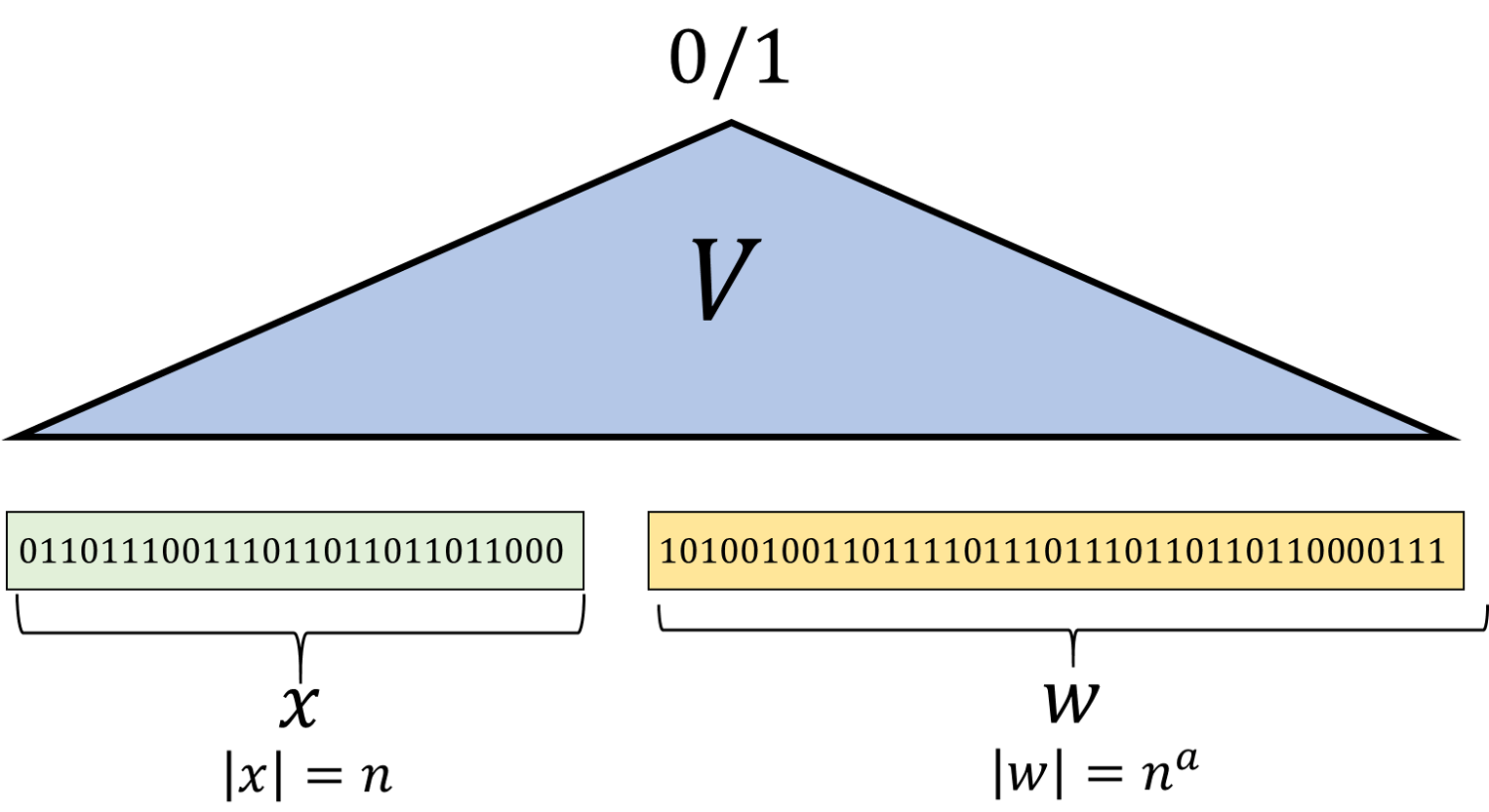
We say that \(F:\{0,1\}^* \rightarrow \{0,1\}\) is in \(\mathbf{NP}\) if there exists some integer \(a>0\) and \(V:\{0,1\}^* \rightarrow \{0,1\}\) such that \(V\in \mathbf{P}\) and for every \(x\in \{0,1\}^n\),
In other words, for \(F\) to be in \(\mathbf{NP}\), there needs to exist some polynomial-time computable verification function \(V\), such that if \(F(x)=1\) then there must exist \(w\) (of length polynomial in \(|x|\)) such that \(V(xw)=1\), and if \(F(x)=0\) then for every such \(w\), \(V(xw)=0\). Since the existence of this string \(w\) certifies that \(F(x)=1\), \(w\) is often referred to as a certificate, witness, or proof that \(F(x)=1\).
See also Figure 15.2 for an illustration of Definition 15.1. The name \(\mathbf{NP}\) stands for “non-deterministic polynomial time” and is used for historical reasons; see the bibiographical notes. The string \(w\) in Equation 15.1 is sometimes known as a solution, certificate, or witness for the instance \(x\).
Show that the condition that \(|w|=|x|^a\) in Definition 15.1 can be replaced by the condition that \(|w| \leq p(|x|)\) for some polynomial \(p\). That is, prove that for every \(F:\{0,1\}^* \rightarrow \{0,1\}\), \(F \in \mathbf{NP}\) if and only if there is a polynomial-time Turing machine \(V\) and a polynomial \(p:\N \rightarrow \N\) such that for every \(x\in \{0,1\}^*\) \(F(x)=1\) if and only if there exists \(w\in \{0,1\}^*\) with \(|w| \leq p(|x|)\) such that \(V(x,w)=1\).
The “only if” direction (namely that if \(F\in \mathbf{NP}\) then there is an algorithm \(V\) and a polynomial \(p\) as above) follows immediately from Definition 15.1 by letting \(p(n)=n^a\). For the “if” direction, the idea is that if a string \(w\) is of size at most \(p(n)\) for degree \(d\) polynomial \(p\), then there is some \(n_0\) such that for all \(n > n_0\), \(|w| < n^{d+1}\). Hence we can encode \(w\) by a string of exactly length \(n^{d+1}\) by padding it with \(1\) and an appropriate number of zeroes. Hence if there is an algorithm \(V\) and polynomial \(p\) as above, then we can define an algorithm \(V'\) that does the following on input \(x,w'\) with \(|x|=n\) and \(|w'|=n^a\):
If \(n \leq n_0\) then \(V'(x,w')\) ignores \(w'\) and enumerates over all \(w\) of length at most \(p(n)\) and outputs \(1\) if there exists \(w\) such that \(V(x,w)=1\). (Since \(n < n_0\), this only takes a constant number of steps.)
If \(n> n_0\) then \(V'(x,w')\) “strips out” the padding by dropping all the rightmost zeroes from \(w\) until it reaches out the first \(1\) (which it drops as well) and obtains a string \(w\). If \(|w| \leq p(n)\) then \(V'\) outputs \(V(x,w)\).
Since \(V\) runs in polynomial time, \(V'\) runs in polynomial time as well, and by definition for every \(x\), there exists \(w' \in \{0,1\}^{|x|^a}\) such that \(V'(xw')=1\) if and only if there exists \(w \in \{0,1\}^*\) with \(|w| \leq p(|x|)\) such that \(V(xw)=1\).
The definition of \(\mathbf{NP}\) means that for every \(F\in \mathbf{NP}\) and string \(x\in \{0,1\}^*\), \(F(x)=1\) if and only if there is a short and efficiently verifiable proof of this fact. That is, we can think of the function \(V\) in Definition 15.1 as a verifier algorithm, similar to what we’ve seen in Section 11.1. The verifier checks whether a given string \(w\in \{0,1\}^*\) is a valid proof for the statement “\(F(x)=1\)”. Essentially all proof systems considered in mathematics involve line-by-line checks that can be carried out in polynomial time. Thus the heart of \(\mathbf{NP}\) is asking for statements that have short (i.e., polynomial in the size of the statements) proofs. Indeed, as we will see in Chapter 16, Kurt Gödel phrased the question of whether \(\mathbf{NP}=\mathbf{P}\) as asking whether “the mental work of a mathematician [in proving theorems] could be completely replaced by a machine”.
Definition 15.1 is asymmetric in the sense that there is a difference between an output of \(1\) and an output of \(0\). You should make sure you understand why this definition does not guarantee that if \(F \in \mathbf{NP}\) then the function \(1-F\) (i.e., the map \(x \mapsto 1-F(x)\)) is in \(\mathbf{NP}\) as well.
In fact, it is believed that there do exist functions \(F\) such that \(F\in \mathbf{NP}\) but \(1-F \not\in \mathbf{NP}\). For example, as shown below, \(3\ensuremath{\mathit{SAT}} \in \mathbf{NP}\), but the function \(\overline{3\ensuremath{\mathit{SAT}}}\) that on input a 3CNF formula \(\varphi\) outputs \(1\) if and only if \(\varphi\) is not satisfiable is not known (nor believed) to be in \(\mathbf{NP}\). This is in contrast to the class \(\mathbf{P}\) which does satisfy that if \(F\in \mathbf{P}\) then \(1-F\) is in \(\mathbf{P}\) as well.
Examples of functions in \(\mathbf{NP}\)
We now present some examples of functions that are in the class \(\mathbf{NP}\). We start with the canonical example of the \(3\ensuremath{\mathit{SAT}}\) function.
\(3\ensuremath{\mathit{SAT}}\) is in \(\mathbf{NP}\) since for every \(\ell\)-variable formula \(\varphi\), \(3\ensuremath{\mathit{SAT}}(\varphi)=1\) if and only if there exists a satisfying assignment \(x \in \{0,1\}^\ell\) such that \(\varphi(x)=1\), and we can check this condition in polynomial time.
The above reasoning explains why \(3\ensuremath{\mathit{SAT}}\) is in \(\mathbf{NP}\), but since this is our first example, we will now belabor the point and expand out in full formality the precise representation of the witness \(w\) and the algorithm \(V\) that demonstrate that \(3\ensuremath{\mathit{SAT}}\) is in \(\mathbf{NP}\). Since demonstrating that functions are in \(\mathbf{NP}\) is fairly straightforward, in future cases we will not use as much detail, and the reader can also feel free to skip the rest of this example.
Using Solved Exercise 15.1, it is OK if witness is of size at most polynomial in the input length \(n\), rather than of precisely size \(n^a\) for some integer \(a>0\). Specifically, we can represent a 3CNF formula \(\varphi\) with \(k\) variables and \(m\) clauses as a string of length \(n=O(m\log k)\), since every one of the \(m\) clauses involves three variables and their negation, and the identity of each variable can be represented using \(\lceil \log_2 k \rceil\). We assume that every variable participates in some clause (as otherwise it can be ignored) and hence that \(m \geq k\), which in particular means that the input length \(n\) is at least as large as \(m\) and \(k\).
We can represent an assignment to the \(k\) variables using a \(k\)-length string \(w\). The following algorithm checks whether a given \(w\) satisfies the formula \(\varphi\):
Algorithm 15.4 Verifier for 3SAT
Input: 3CNF formula \(\varphi\) on \(k\) variables and with \(m\) clauses, string \(w \in \{0,1\}^k\)
Output: \(1\) iff \(w\) satisfies \(\varphi\)
for{\(j \in [m]\)}
Let \(\ell_1 \vee \ell_2 \vee \ell_3\) be the \(j\)-th clause of \(\varphi\)
if{\(w\) violates all three literals}
return \(0\)
endif
endfor
return \(1\)
Algorithm 15.4 takes \(O(m)\) time to enumerate over all clauses, and will return \(1\) if and only if \(y\) satisfies all the clauses.
Here are some more examples for problems in \(\mathbf{NP}\). For each one of these problems we merely sketch how the witness is represented and why it is efficiently checkable, but working out the details can be a good way to get more comfortable with Definition 15.1:
\(\ensuremath{\mathit{QUADEQ}}\) is in \(\mathbf{NP}\) since for every \(\ell\)-variable instance of quadratic equations \(E\), \(\ensuremath{\mathit{QUADEQ}}(E)=1\) if and only if there exists an assignment \(x\in \{0,1\}^\ell\) that satisfies \(E\). We can check the condition that \(x\) satisfies \(E\) in polynomial time by enumerating over all the equations in \(E\), and for each such equation \(e\), plug in the values of \(x\) and verify that \(e\) is satisfied.
\(\ensuremath{\mathit{ISET}}\) is in \(\mathbf{NP}\) since for every graph \(G\) and integer \(k\), \(\ensuremath{\mathit{ISET}}(G,k)=1\) if and only if there exists a set \(S\) of \(k\) vertices that contains no pair of neighbors in \(G\). We can check the condition that \(S\) is an independent set of size \(\geq k\) in polynomial time by first checking that \(|S| \geq k\) and then enumerating over all edges \(\{u,v \}\) in \(G\), and for each such edge verify that either \(u\not\in S\) or \(v\not\in S\).
\(\ensuremath{\mathit{LONGPATH}}\) is in \(\mathbf{NP}\) since for every graph \(G\) and integer \(k\), \(\ensuremath{\mathit{LONGPATH}}(G,k)=1\) if and only if there exists a simple path \(P\) in \(G\) that is of length at least \(k\). We can check the condition that \(P\) is a simple path of length \(k\) in polynomial time by checking that it has the form \((v_0,v_1,\ldots,v_k)\) where each \(v_i\) is a vertex in \(G\), no \(v_i\) is repeated, and for every \(i \in [k]\), the edge \(\{v_i,v_{i+1}\}\) is present in the graph.
\(\ensuremath{\mathit{MAXCUT}}\) is in \(\mathbf{NP}\) since for every graph \(G\) and integer \(k\), \(\ensuremath{\mathit{MAXCUT}}(G,k)=1\) if and only if there exists a cut \((S,\overline{S})\) in \(G\) that cuts at least \(k\) edges. We can check that condition that \((S,\overline{S})\) is a cut of value at least \(k\) in polynomial time by checking that \(S\) is a subset of \(G\)’s vertices and enumerating over all the edges \(\{u,v\}\) of \(G\), counting those edges such that \(u\in S\) and \(v\not\in S\) or vice versa.
Basic facts about \(\mathbf{NP}\)
The definition of \(\mathbf{NP}\) is one of the most important definitions of this book, and is worth while taking the time to digest and internalize. The following solved exercises establish some basic properties of this class. As usual, I highly recommend that you try to work out the solutions yourself.
Prove that \(\mathbf{P} \subseteq \mathbf{NP}\).
Suppose that \(F \in \mathbf{P}\). Define the following function \(V\): \(V(x0^n)=1\) iff \(n=|x|\) and \(F(x)=1\). (\(V\) outputs \(0\) on all other inputs.) Since \(F\in \mathbf{P}\) we can clearly compute \(V\) in polynomial time as well.
Let \(x\in \{0,1\}^n\) be some string. If \(F(x)=1\) then \(V(x0^n)=1\). On the other hand, if \(F(x)=0\) then for every \(w\in \{0,1\}^n\), \(V(xw)=0\). Therefore, setting \(a=1\) (i.e. \(w\in \{0,1\}^{n^1}\)), we see that \(V\) satisfies Equation 15.1, and establishes that \(F \in \mathbf{NP}\).
People sometimes think that \(\mathbf{NP}\) stands for “non-polynomial time”. As Solved Exercise 15.2 shows, this is far from the truth, and in fact every polynomial-time computable function is in \(\mathbf{NP}\) as well.
If \(F\) is in \(\mathbf{NP}\) it certainly does not mean that \(F\) is hard to compute (though it does not, as far as we know, necessarily mean that it’s easy to compute either). Rather, it means that \(F\) is easy to verify, in the technical sense of Definition 15.1.
Prove that \(\mathbf{NP} \subseteq \mathbf{EXP}\).
Suppose that \(F\in \mathbf{NP}\) and let \(V\) be the polynomial-time computable function that satisfies Equation 15.1 and \(a\) the corresponding constant. Then given every \(x\in \{0,1\}^n\), we can check whether \(F(x)=1\) in time \(poly(n)\cdot 2^{n^a} = o(2^{n^{a+1}})\) by enumerating over all the \(2^{n^a}\) strings \(w\in \{0,1\}^{n^a}\) and checking whether \(V(xw)=1\), in which case we return \(1\). If \(V(xw)=0\) for every such \(w\) then we return \(0\). By construction, the algorithm above will run in time at most exponential in its input length and by the definition of \(\mathbf{NP}\) it will return \(F(x)\) for every \(x\).
Solved Exercise 15.2 and Solved Exercise 15.3 together imply that
The time hierarchy theorem (Theorem 13.9) implies that \(\mathbf{P} \subsetneq \mathbf{EXP}\) and hence at least one of the two inclusions \(\mathbf{P} \subseteq \mathbf{NP}\) or \(\mathbf{NP} \subseteq \mathbf{EXP}\) is strict. It is believed that both of them are in fact strict inclusions. That is, it is believed that there are functions in \(\mathbf{NP}\) that cannot be computed in polynomial time (this is the \(\mathbf{P} \neq \mathbf{NP}\) conjecture) and that there are functions \(F\) in \(\mathbf{EXP}\) for which we cannot even efficiently certify that \(F(x)=1\) for a given input \(x\). One function \(F\) that is believed to lie in \(\mathbf{EXP} \setminus \mathbf{NP}\) is the function \(\overline{3\ensuremath{\mathit{SAT}}}\) defined as \(\overline{3\ensuremath{\mathit{SAT}}}(\varphi)= 1 - 3\ensuremath{\mathit{SAT}}(\varphi)\) for every 3CNF formula \(\varphi\). The conjecture that \(\overline{3\ensuremath{\mathit{SAT}}}\not\in \mathbf{NP}\) is known as the “\(\mathbf{NP} \neq \mathbf{co-NP}\)” conjecture. It implies the \(\mathbf{P} \neq \mathbf{NP}\) conjecture (see Exercise 15.2).
We have previously informally equated the notion of \(F \leq_p G\) with \(F\) being “no harder than \(G\)” and in particular have seen in Solved Exercise 14.1 that if \(G \in \mathbf{P}\) and \(F \leq_p G\), then \(F \in \mathbf{P}\) as well. The following exercise shows that if \(F \leq_p G\) then it is also “no harder to verify” than \(G\). That is, regardless of whether or not it is in \(\mathbf{P}\), if \(G\) has the property that solutions to it can be efficiently verified, then so does \(F\).
Let \(F,G:\{0,1\}^* \rightarrow \{0,1\}\). Show that if \(F \leq_p G\) and \(G\in \mathbf{NP}\) then \(F \in \mathbf{NP}\).
Suppose that \(G\) is in \(\mathbf{NP}\) and in particular there exists \(a\) and \(V \in \mathbf{P}\) such that for every \(y \in \{0,1\}^*\), \(G(y)=1 \Leftrightarrow \exists_{w\in \{0,1\}^{|y|^a}} V(yw)=1\). Suppose also that \(F \leq_p G\) and so in particular there is a \(n^b\)-time computable function \(R\) such that \(F(x) = G(R(x))\) for all \(x\in \{0,1\}^*\). Define \(V'\) to be a Turing machine that on input a pair \((x,w)\) computes \(y=R(x)\) and returns \(1\) if and only if \(|w|=|y|^a\) and \(V(yw)=1\). Then \(V'\) runs in polynomial time, and for every \(x\in \{0,1\}^*\), \(F(x)=1\) iff there exists \(w\) of size \(|R(x)|^a\) which is at most polynomial in \(|x|\) such that \(V'(x,w)=1\), hence demonstrating that \(F \in \mathbf{NP}\).
From \(\mathbf{NP}\) to 3SAT: The Cook-Levin Theorem
We have seen several examples of problems for which we do not know if their best algorithm is polynomial or exponential, but we can show that they are in \(\mathbf{NP}\). That is, we don’t know if they are easy to solve, but we do know that it is easy to verify a given solution. There are many, many, many, more examples of interesting functions we would like to compute that are easily shown to be in \(\mathbf{NP}\). What is quite amazing is that if we can solve 3SAT then we can solve all of them!
The following is one of the most fundamental theorems in Computer Science:
For every \(F\in \mathbf{NP}\), \(F \leq_p 3\ensuremath{\mathit{SAT}}\).
We will soon show the proof of Theorem 15.6, but note that it immediately implies that \(\ensuremath{\mathit{QUADEQ}}\), \(\ensuremath{\mathit{LONGPATH}}\), and \(\ensuremath{\mathit{MAXCUT}}\) all reduce to \(3\ensuremath{\mathit{SAT}}\). Combining it with the reductions we’ve seen in Chapter 14, it implies that all these problems are equivalent! For example, to reduce \(\ensuremath{\mathit{QUADEQ}}\) to \(\ensuremath{\mathit{LONGPATH}}\), we can first reduce \(\ensuremath{\mathit{QUADEQ}}\) to \(3\ensuremath{\mathit{SAT}}\) using Theorem 15.6 and use the reduction we’ve seen in Theorem 14.12 from \(3\ensuremath{\mathit{SAT}}\) to \(\ensuremath{\mathit{LONGPATH}}\). That is, since \(\ensuremath{\mathit{QUADEQ}} \in \mathbf{NP}\), Theorem 15.6 implies that \(\ensuremath{\mathit{QUADEQ}} \leq_p 3\ensuremath{\mathit{SAT}}\), and Theorem 14.12 implies that \(3\ensuremath{\mathit{SAT}} \leq_p \ensuremath{\mathit{LONGPATH}}\), which by the transitivity of reductions (Solved Exercise 14.2) means that \(\ensuremath{\mathit{QUADEQ}} \leq_p \ensuremath{\mathit{LONGPATH}}\). Similarly, since \(\ensuremath{\mathit{LONGPATH}} \in \mathbf{NP}\), we can use Theorem 15.6 and Theorem 14.4 to show that \(\ensuremath{\mathit{LONGPATH}} \leq_p 3\ensuremath{\mathit{SAT}} \leq_p \ensuremath{\mathit{QUADEQ}}\), concluding that \(\ensuremath{\mathit{LONGPATH}}\) and \(\ensuremath{\mathit{QUADEQ}}\) are computationally equivalent.
There is of course nothing special about \(\ensuremath{\mathit{QUADEQ}}\) and \(\ensuremath{\mathit{LONGPATH}}\) here: by combining Theorem 15.6 with the reductions we saw, we see that just like \(3\ensuremath{\mathit{SAT}}\), every \(F\in \mathbf{NP}\) reduces to \(\ensuremath{\mathit{LONGPATH}}\), and the same is true for \(\ensuremath{\mathit{QUADEQ}}\) and \(\ensuremath{\mathit{MAXCUT}}\). All these problems are in some sense “the hardest in \(\mathbf{NP}\)” since an efficient algorithm for any one of them would imply an efficient algorithm for all the problems in \(\mathbf{NP}\). This motivates the following definition:
Let \(G:\{0,1\}^* \rightarrow \{0,1\}\). We say that \(G\) is \(\mathbf{NP}\) hard if for every \(F\in \mathbf{NP}\), \(F \leq_p G\).
We say that \(G\) is \(\mathbf{NP}\) complete if \(G\) is \(\mathbf{NP}\) hard and \(G \in \mathbf{NP}\).
The Cook-Levin Theorem (Theorem 15.6) can be rephrased as saying that \(3\ensuremath{\mathit{SAT}}\) is \(\mathbf{NP}\) hard, and since it is also in \(\mathbf{NP}\), this means that \(3\ensuremath{\mathit{SAT}}\) is \(\mathbf{NP}\) complete. Together with the reductions of Chapter 14, Theorem 15.6 shows that despite their superficial differences, 3SAT, quadratic equations, longest path, independent set, and maximum cut, are all \(\mathbf{NP}\)-complete. Many thousands of additional problems have been shown to be \(\mathbf{NP}\)-complete, arising from all the sciences, mathematics, economics, engineering and many other fields. (For a few examples, see this Wikipedia page and this website.)
If a single \(\mathbf{NP}\)-complete has a polynomial-time algorithm, then there is such an algorithm for every decision problem that corresponds to the existence of an efficiently-verifiable solution.
What does this mean?
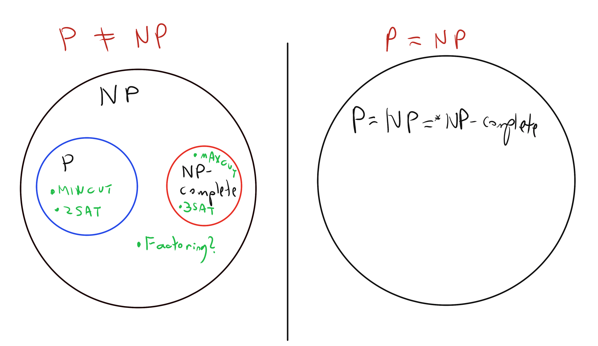
As we’ve seen in Solved Exercise 15.2, \(\mathbf{P} \subseteq \mathbf{NP}\). The most famous conjecture in Computer Science is that this containment is strict. That is, it is widely conjectured that \(\mathbf{P} \neq \mathbf{NP}\). One way to refute the conjecture that \(\mathbf{P} \neq \mathbf{NP}\) is to give a polynomial-time algorithm for even a single one of the \(\mathbf{NP}\)-complete problems such as 3SAT, Max Cut, or the thousands of others that have been studied in all fields of human endeavors. The fact that these problems have been studied by so many people, and yet not a single polynomial-time algorithm for any of them has been found, supports that conjecture that indeed \(\mathbf{P} \neq \mathbf{NP}\). In fact, for many of these problems (including all the ones we mentioned above), we don’t even know of a \(2^{o(n)}\)-time algorithm! However, to the frustration of computer scientists, we have not yet been able to prove that \(\mathbf{P}\neq\mathbf{NP}\) or even rule out the existence of an \(O(n)\)-time algorithm for 3SAT. Resolving whether or not \(\mathbf{P}=\mathbf{NP}\) is known as the \(\mathbf{P}\) vs \(\mathbf{NP}\) problem. A million-dollar prize has been offered for the solution of this problem, a popular book has been written, and every year a new paper comes out claiming a proof of \(\mathbf{P}=\mathbf{NP}\) or \(\mathbf{P}\neq\mathbf{NP}\), only to wither under scrutiny.
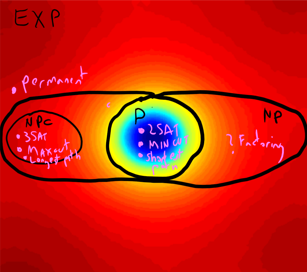
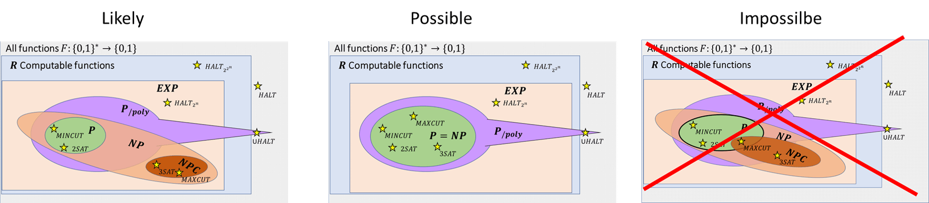
One of the mysteries of computation is that people have observed a certain empirical “zero-one law” or “dichotomy” in the computational complexity of natural problems, in the sense that many natural problems are either in \(\mathbf{P}\) (often in \(\ensuremath{\mathit{TIME}}(O(n))\) or \(\ensuremath{\mathit{TIME}}(O(n^2))\)), or they are are \(\mathbf{NP}\) hard. This is related to the fact that for most natural problems, the best known algorithm is either exponential or polynomial, with not too many examples where the best running time is some strange intermediate complexity such as \(2^{2^{\sqrt{\log n}}}\). However, it is believed that there exist problems in \(\mathbf{NP}\) that are neither in \(\mathbf{P}\) nor are \(\mathbf{NP}\)-complete, and in fact a result known as “Ladner’s Theorem” shows that if \(\mathbf{P} \neq \mathbf{NP}\) then this is indeed the case (see also Exercise 15.1 and Figure 15.3).
The Cook-Levin Theorem: Proof outline
We will now prove the Cook-Levin Theorem, which is the underpinning to a great web of reductions from 3SAT to thousands of problems across many great fields. Some problems that have been shown to be \(\mathbf{NP}\)-complete include: minimum-energy protein folding, minimum surface-area foam configuration, map coloring, optimal Nash equilibrium, quantum state entanglement, minimum supersequence of a genome, minimum codeword problem, shortest vector in a lattice, minimum genus knots, positive Diophantine equations, integer programming, and many many more. The worst-case complexity of all these problems is (up to polynomial factors) equivalent to that of 3SAT, and through the Cook-Levin Theorem, to all problems in \(\mathbf{NP}\).
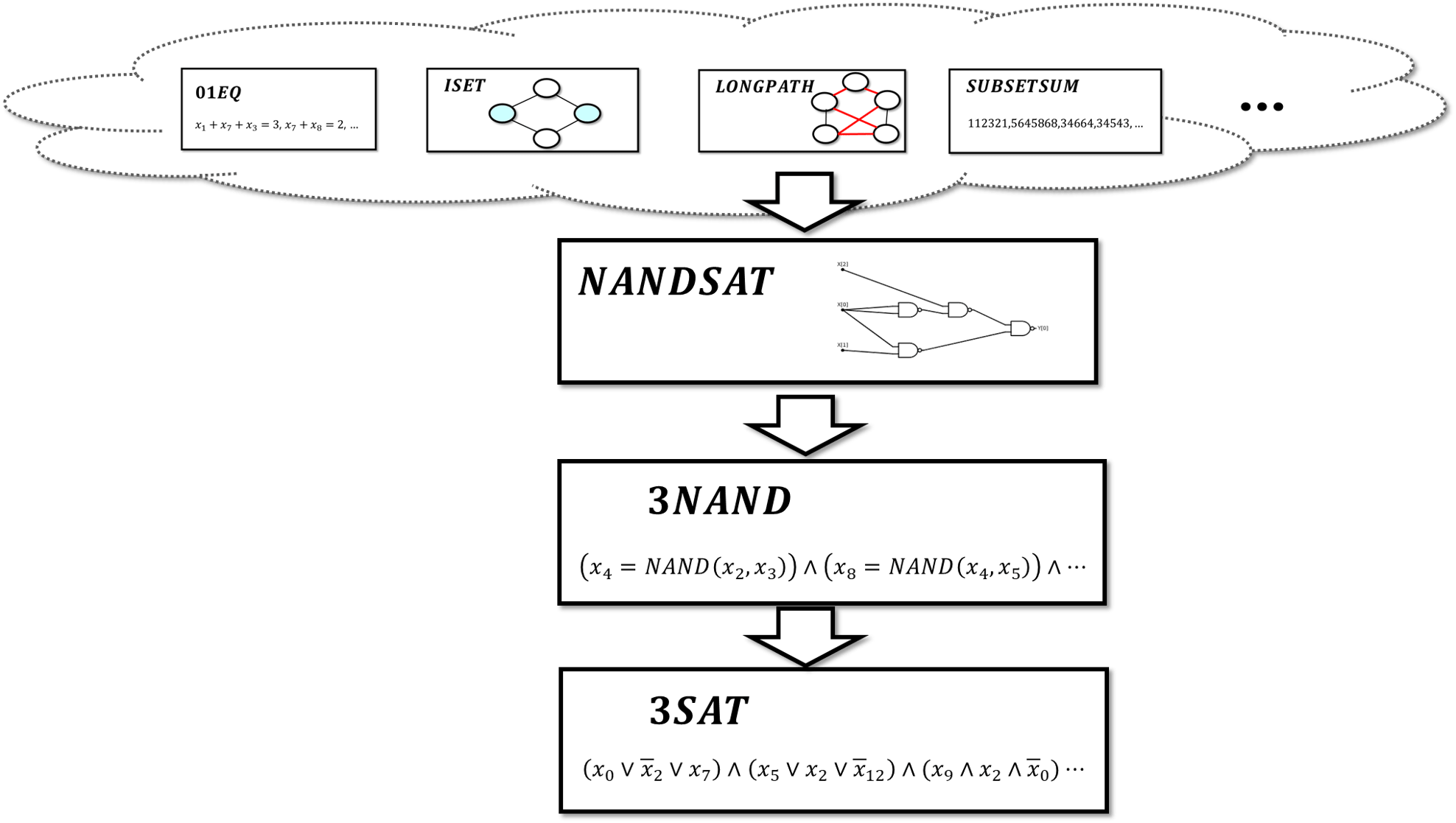
To prove Theorem 15.6 we need to show that \(F \leq_p 3\ensuremath{\mathit{SAT}}\) for every \(F\in \mathbf{NP}\). We will do so in three stages. We define two intermediate problems: \(\ensuremath{\mathit{NANDSAT}}\) and \(3\ensuremath{\mathit{NAND}}\). We will shortly show the definitions of these two problems, but Theorem 15.6 will follow from combining the following three results:
\(\ensuremath{\mathit{NANDSAT}}\) is \(\mathbf{NP}\) hard (Lemma 15.8).
\(\ensuremath{\mathit{NANDSAT}} \leq_p 3\ensuremath{\mathit{NAND}}\) (Lemma 15.9).
\(3\ensuremath{\mathit{NAND}} \leq_p 3\ensuremath{\mathit{SAT}}\) (Lemma 15.10).
By the transitivity of reductions, it will follow that for every \(F \in \mathbf{NP}\),
hence establishing Theorem 15.6.
We will prove these three results Lemma 15.8, Lemma 15.9 and Lemma 15.10 one by one, providing the requisite definitions as we go along.
The \(\ensuremath{\mathit{NANDSAT}}\) Problem, and why it is \(\mathbf{NP}\) hard
The function \(\ensuremath{\mathit{NANDSAT}}:\{0,1\}^* \rightarrow \{0,1\}\) is defined as follows:
The input to \(\ensuremath{\mathit{NANDSAT}}\) is a string \(Q\) representing a NAND-CIRC program (or equivalently, a circuit with NAND gates).
The output of \(\ensuremath{\mathit{NANDSAT}}\) on input \(Q\) is \(1\) if and only if there exists a string \(w\in \{0,1\}^n\) (where \(n\) is the number of inputs to \(Q\)) such that \(Q(w)=1\).
Prove that \(\ensuremath{\mathit{NANDSAT}} \in \mathbf{NP}\).
We have seen that the circuit (or straightline program) evaluation problem can be computed in polynomial time. Specifically, given a NAND-CIRC program \(Q\) of \(s\) lines and \(n\) inputs, and \(w\in \{0,1\}^n\), we can evaluate \(Q\) on the input \(w\) in time which is polynomial in \(s\) and hence verify whether or not \(Q(w)=1\).
We now prove that \(\ensuremath{\mathit{NANDSAT}}\) is \(\mathbf{NP}\) hard.
\(\ensuremath{\mathit{NANDSAT}}\) is \(\mathbf{NP}\) hard.
The proof closely follows the proof that \(\mathbf{P} \subseteq \mathbf{P_{/poly}}\) (Theorem 13.12 , see also Section 13.6.2). Specifically, if \(F\in \mathbf{NP}\) then there is a polynomial time Turing machine \(M\) and positive integer \(a\) such that for every \(x\in \{0,1\}^n\), \(F(x)=1\) iff there is some \(w \in \{0,1\}^{n^a}\) such that \(M(xw)=1\). The proof that \(\mathbf{P} \subseteq \mathbf{P_{/poly}}\) gave us a way (via “unrolling the loop”) to come up in polynomial time with a Boolean circuit \(C\) on \(n^a\) inputs that computes the function \(w \mapsto M(xw)\). We can then translate \(C\) into an equivalent NAND circuit (or NAND-CIRC program) \(Q\). We see that there is a string \(w \in \{0,1\}^{n^a}\) such that \(Q(w)=1\) if and only if there is such \(w\) satisfying \(M(xw)=1\) which (by definition) happens if and only if \(F(x)=1\). Hence the translation of \(x\) into the circuit \(Q\) is a reduction showing \(F \leq_p \ensuremath{\mathit{NANDSAT}}\).
The proof is a little bit technical but ultimately follows quite directly from the definition of \(\mathbf{NP}\), as well as the ability to “unroll the loop” of NAND-TM programs as discussed in Section 13.6.2. If you find it confusing, try to pause here and think how you would implement in your favorite programming language the function unroll which on input a NAND-TM program \(P\) and numbers \(T,n\) outputs an \(n\)-input NAND-CIRC program \(Q\) of \(O(|T|)\) lines such that for every input \(z\in \{0,1\}^n\), if \(P\) halts on \(z\) within at most \(T\) steps and outputs \(y\), then \(Q(z)=y\).
Let \(F \in \mathbf{NP}\). To prove Lemma 15.8 we need to give a polynomial-time computable function that will map every \(x^* \in \{0,1\}^*\) to a NAND-CIRC program \(Q\) such that \(F(x^*)=\ensuremath{\mathit{NANDSAT}}(Q)\).
Let \(x^* \in \{0,1\}^*\) be such a string and let \(n=|x^*|\) be its length. By Definition 15.1 there exists \(V \in \mathbf{P}\) and positive \(a \in \N\) such that \(F(x^*)=1\) if and only if there exists \(w\in \{0,1\}^{n^a}\) satisfying \(V(x^*w)=1\).
Let \(m=n^a\). Since \(V\in \mathbf{P}\) there is some NAND-TM program \(P^*\) that computes \(V\) on inputs of the form \(xw\) with \(x\in \{0,1\}^n\) and \(w\in \{0,1\}^m\) in at most \({(n+m)}^c\) time for some constant \(c\). Using our “unrolling the loop NAND-TM to NAND compiler” of Theorem 13.14, we can obtain a NAND-CIRC program \(Q'\) that has \(n+m\) inputs and at most \(O((n+m)^{2c})\) lines such that \(Q'(xw)= P^*(xw)\) for every \(x\in \{0,1\}^n\) and \(w \in \{0,1\}^m\).
We can then use a simple “hardwiring” technique, reminiscent of Remark 9.11 to map \(Q'\) into a circuit/NAND-CIRC program \(Q\) on \(m\) inputs such that \(Q(w)= Q'(x^*w)\) for every \(w\in \{0,1\}^m\).
CLAIM: There is a polynomial-time algorithm that on input a NAND-CIRC program \(Q'\) on \(n+m\) inputs and \(x^* \in \{0,1\}^n\), outputs a NAND-CIRC program \(Q\) such that for every \(w\in \{0,1\}^n\), \(Q(w)=Q'(x^*w)\).
PROOF OF CLAIM: We can do so by adding a few lines to ensure that the variables zero and one are \(0\) and \(1\) respectively, and then simply replacing any reference in \(Q'\) to an input \(x_i\) with \(i\in [n]\) the corresponding value based on \(x^*_i\). See Figure 15.5 for an implementation of this reduction in Python.
Our final reduction maps an input \(x^*\), into the NAND-CIRC program \(Q\) obtained above. By the above discussion, this reduction runs in polynomial time. Since we know that \(F(x^*)=1\) if and only if there exists \(w\in \{0,1\}^m\) such that \(P^*(x^*w)=1\), this means that \(F(x^*)=1\) if and only if \(\ensuremath{\mathit{NANDSAT}}(Q)=1\), which is what we wanted to prove.
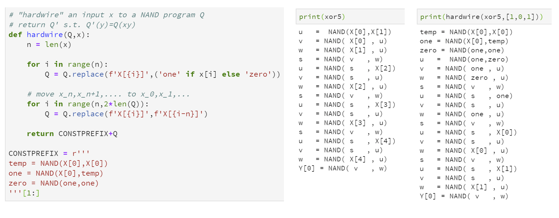
zero and one constants, replacing all references to X[\(i\)] with either zero or one depending on the value of \(x^*_i\), and then replacing the remaining references to X[\(j\)] with X[\(j-n\)]. Above is Python code that implements this transformation, as well as an example of its execution on a simple program.The \(3\ensuremath{\mathit{NAND}}\) problem
The \(3\ensuremath{\mathit{NAND}}\) problem is defined as follows:
The input is a logical formula \(\Psi\) on a set of variables \(z_0,\ldots,z_{r-1}\) which is an AND of constraints of the form \(z_i = \ensuremath{\mathit{NAND}}(z_j,z_k)\).
The output is \(1\) if and only if there is an input \(z\in \{0,1\}^r\) that satisfies all of the constraints.
For example, the following is a \(3\ensuremath{\mathit{NAND}}\) formula with \(5\) variables and \(3\) constraints:
In this case \(3\ensuremath{\mathit{NAND}}(\Psi)=1\) since the assignment \(z = 01010\) satisfies it. Given a \(3\ensuremath{\mathit{NAND}}\) formula \(\Psi\) on \(r\) variables and an assignment \(z\in \{0,1\}^r\), we can check in polynomial time whether \(\Psi(z)=1\), and hence \(3\ensuremath{\mathit{NAND}} \in \mathbf{NP}\). We now prove that \(3\ensuremath{\mathit{NAND}}\) is \(\mathbf{NP}\) hard:
\(\ensuremath{\mathit{NANDSAT}} \leq_p 3\ensuremath{\mathit{NAND}}\).
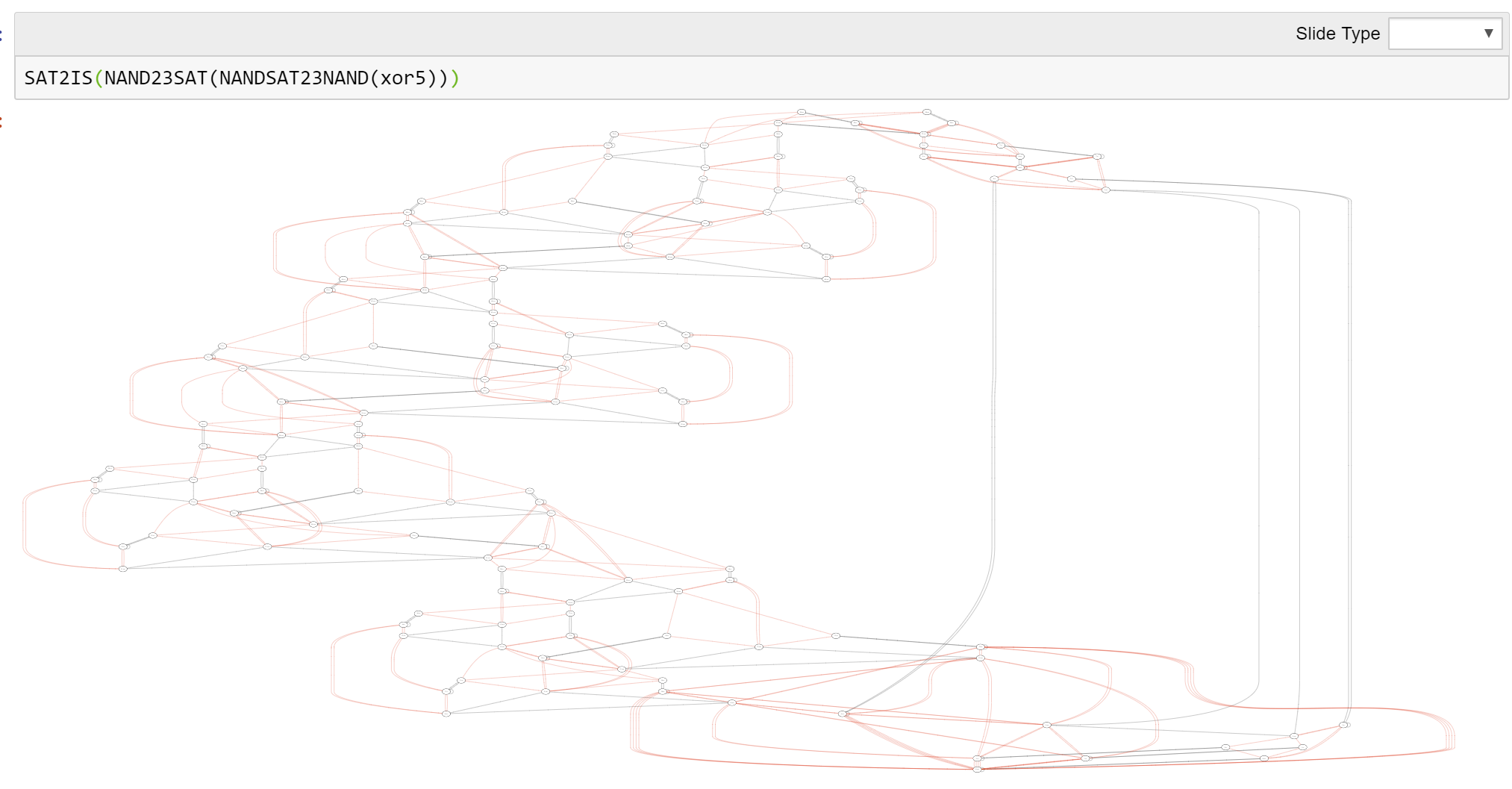
To prove Lemma 15.9 we need to give a polynomial-time map from every NAND-CIRC program \(Q\) to a 3NAND formula \(\Psi\) such that there exists \(w\) such that \(Q(w)=1\) if and only if there exists \(z\) satisfying \(\Psi\). For every line \(i\) of \(Q\), we define a corresponding variable \(z_i\) of \(\Psi\). If the line \(i\) has the form foo = NAND(bar,blah) then we will add the clause \(z_i = \ensuremath{\mathit{NAND}}(z_j,z_k)\) where \(j\) and \(k\) are the last lines in which bar and blah were written to. We will also set variables corresponding to the input variables, as well as add a clause to ensure that the final output is \(1\). The resulting reduction can be implemented in about a dozen lines of Python, see Figure 15.6.
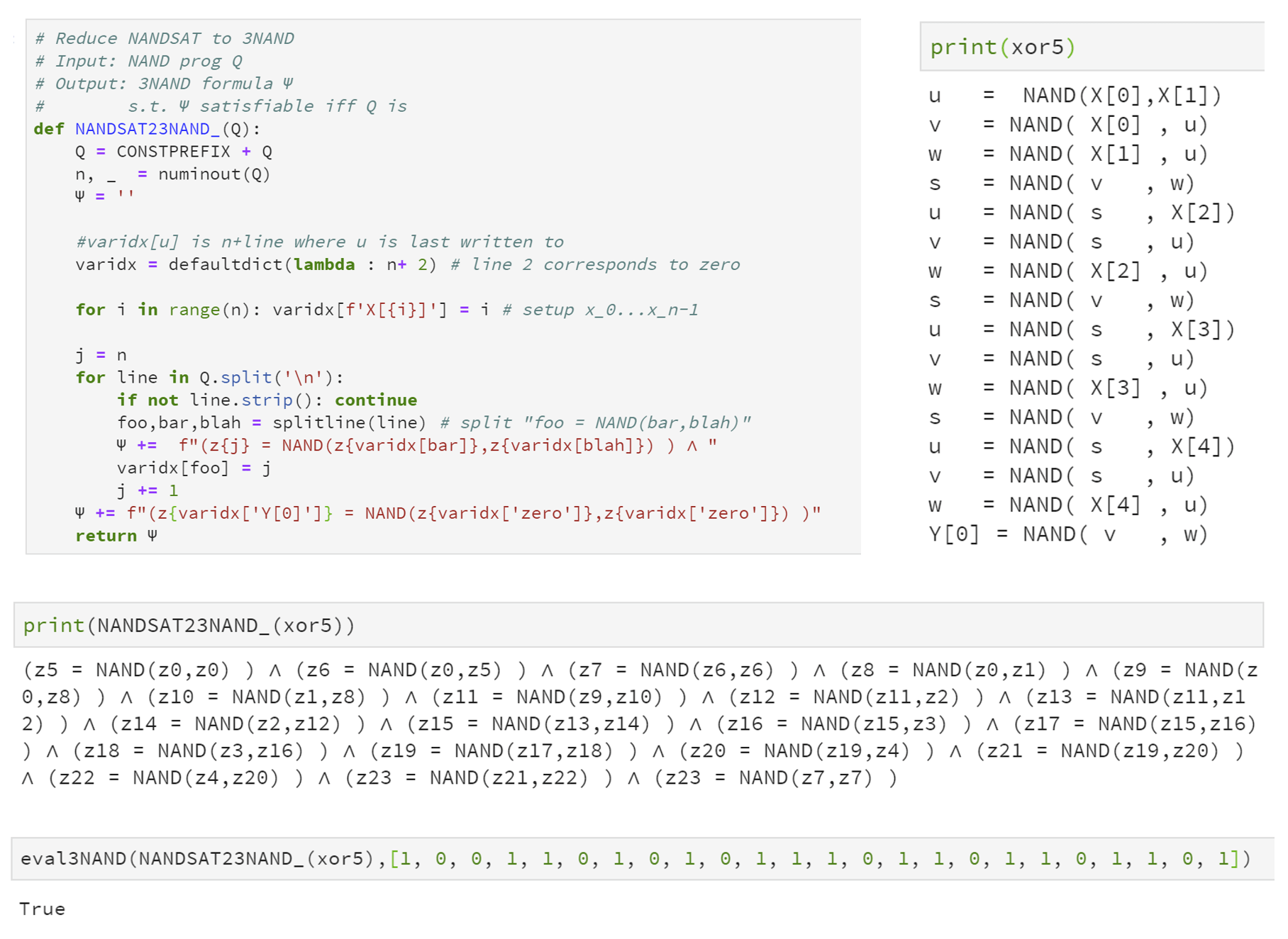
xor5 which has \(5\) input variables and \(16\) lines, into a \(3\ensuremath{\mathit{NAND}}\) formula \(\Psi\) that has \(24\) variables and \(20\) clauses. Since xor5 outputs \(1\) on the input \(1,0,0,1,1\), there exists an assignment \(z \in \{0,1\}^{24}\) to \(\Psi\) such that \((z_0,z_1,z_2,z_3,z_4)=(1,0,0,1,1)\) and \(\Psi\) evaluates to true on \(z\).To prove Lemma 15.9 we need to give a reduction from \(\ensuremath{\mathit{NANDSAT}}\) to \(3\ensuremath{\mathit{NAND}}\). Let \(Q\) be a NAND-CIRC program with \(n\) inputs, one output, and \(m\) lines. We can assume without loss of generality that \(Q\) contains the variables one and zero as usual.
We map \(Q\) to a \(3\ensuremath{\mathit{NAND}}\) formula \(\Psi\) as follows:
\(\Psi\) has \(m+n\) variables \(z_0,\ldots,z_{m+n-1}\).
The first \(n\) variables \(z_0,\ldots,z_{n-1}\) will corresponds to the inputs of \(Q\). The next \(m\) variables \(z_n,\ldots,z_{n+m-1}\) will correspond to the \(m\) lines of \(Q\).
For every \(\ell\in \{n,n+1,\ldots,n+m \}\), if the \(\ell-n\)-th line of the program \(Q\) is
foo = NAND(bar,blah)then we add to \(\Psi\) the constraint \(z_\ell = \ensuremath{\mathit{NAND}}(z_j,z_k)\) where \(j-n\) and \(k-n\) correspond to the last lines in which the variablesbarandblah(respectively) were written to. If one or both ofbarandblahwas not written to before then we use \(z_{\ell_0}\) instead of the corresponding value \(z_j\) or \(z_k\) in the constraint, where \(\ell_0-n\) is the line in whichzerois assigned a value. If one or both ofbarandblahis an input variableX[i]then we use \(z_i\) in the constraint.Let \(\ell^*\) be the last line in which the output
y_0is assigned a value. Then we add the constraint \(z_{\ell^*} = \ensuremath{\mathit{NAND}}(z_{\ell_0},z_{\ell_0})\) where \(\ell_0-n\) is as above the last line in whichzerois assigned a value. Note that this is effectively the constraint \(z_{\ell^*}=\ensuremath{\mathit{NAND}}(0,0)=1\).
To complete the proof we need to show that there exists \(w\in \{0,1\}^n\) s.t. \(Q(w)=1\) if and only if there exists \(z\in \{0,1\}^{n+m}\) that satisfies all constraints in \(\Psi\). We now show both sides of this equivalence.
Part I: Completeness. Suppose that there is \(w\in \{0,1\}^n\) s.t. \(Q(w)=1\). Let \(z\in \{0,1\}^{n+m}\) be defined as follows: for \(i\in [n]\), \(z_i=w_i\) and for \(i\in \{n,n+1,\ldots,n+m\}\) \(z_i\) equals the value that is assigned in the \((i-n)\)-th line of \(Q\) when executed on \(w\). Then by construction \(z\) satisfies all of the constraints of \(\Psi\) (including the constraint that \(z_{\ell^*}=\ensuremath{\mathit{NAND}}(0,0)=1\) since \(Q(w)=1\).)
Part II: Soundness. Suppose that there exists \(z\in \{0,1\}^{n+m}\) satisfying \(\Psi\). Soundness will follow by showing that \(Q(z_0,\ldots,z_{n-1})=1\) (and hence in particular there exists \(w\in \{0,1\}^n\), namely \(w=z_0\cdots z_{n-1}\), such that \(Q(w)=1\)). To do this we will prove the following claim \((*)\): for every \(\ell \in [m]\), \(z_{\ell+n}\) equals the value assigned in the \(\ell\)-th step of the execution of the program \(Q\) on \(z_0,\ldots,z_{n-1}\). Note that because \(z\) satisfies the constraints of \(\Psi\), \((*)\) is sufficient to prove the soundness condition since these constraints imply that the last value assigned to the variable y_0 in the execution of \(Q\) on \(z_0\cdots z_{n-1}\) is equal to \(1\). To prove \((*)\) suppose, towards a contradiction, that it is false, and let \(\ell\) be the smallest number such that \(z_{\ell+n}\) is not equal to the value assigned in the \(\ell\)-th step of the execution of \(Q\) on \(z_0,\ldots,z_{n-1}\). But since \(z\) satisfies the constraints of \(\Psi\), we get that \(z_{\ell+n}=\ensuremath{\mathit{NAND}}(z_i,z_j)\) where (by the assumption above that \(\ell\) is smallest with this property) these values do correspond to the values last assigned to the variables on the right-hand side of the assignment operator in the \(\ell\)-th line of the program. But this means that the value assigned in the \(\ell\)-th step is indeed simply the NAND of \(z_i\) and \(z_j\), contradicting our assumption on the choice of \(\ell\).
From \(3\ensuremath{\mathit{NAND}}\) to \(3\ensuremath{\mathit{SAT}}\)
The final step in the proof of Theorem 15.6 is the following:
\(3\ensuremath{\mathit{NAND}} \leq_p 3\ensuremath{\mathit{SAT}}\).
To prove Lemma 15.10 we need to map a 3NAND formula \(\varphi\) into a 3SAT formula \(\psi\) such that \(\varphi\) is satisfiable if and only if \(\psi\) is. The idea is that we can transform every NAND constraint of the form \(a=\ensuremath{\mathit{NAND}}(b,c)\) into the AND of ORs involving the variables \(a,b,c\) and their negations, where each of the ORs contains at most three terms. The construction is fairly straightforward, and the details are given below.
It is a good exercise for you to try to find a 3CNF formula \(\xi\) on three variables \(a,b,c\) such that \(\xi(a,b,c)\) is true if and only if \(a = \ensuremath{\mathit{NAND}}(b,c)\). Once you do so, try to see why this implies a reduction from \(3\ensuremath{\mathit{NAND}}\) to \(3\ensuremath{\mathit{SAT}}\), and hence completes the proof of Lemma 15.10
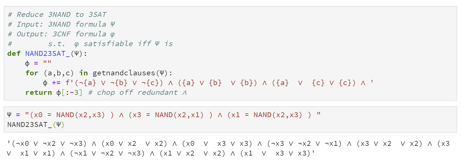
The constraint is satisfied if \(z_i=1\) whenever \((z_j,z_k) \neq (1,1)\). By going through all cases, we can verify that Equation 15.2 is equivalent to the constraint
Indeed if \(z_j=z_k=1\) then the first constraint of Equation 15.3 is only true if \(z_i=0\). On the other hand, if either of \(z_j\) or \(z_k\) equals \(0\) then unless \(z_i=1\) either the second or third constraints will fail. This means that, given any 3NAND formula \(\varphi\) over \(n\) variables \(z_0,\ldots,z_{n-1}\), we can obtain a 3SAT formula \(\psi\) over the same variables by replacing every \(3\ensuremath{\mathit{NAND}}\) constraint of \(\varphi\) with three \(3\ensuremath{\mathit{OR}}\) constraints as in Equation 15.3.1 Because of the equivalence of Equation 15.2 and Equation 15.3, the formula \(\psi\) satisfies that \(\psi(z_0,\ldots,z_{n-1})=\varphi(z_0,\ldots,z_{n-1})\) for every assignment \(z_0,\ldots,z_{n-1} \in \{0,1\}^n\) to the variables. In particular \(\psi\) is satisfiable if and only if \(\varphi\) is, thus completing the proof.
xor5 NAND-CIRC program.Wrapping up
We have shown that for every function \(F\) in \(\mathbf{NP}\), \(F \leq_p \ensuremath{\mathit{NANDSAT}} \leq_p 3\ensuremath{\mathit{NAND}} \leq_p 3\ensuremath{\mathit{SAT}}\), and so \(3\ensuremath{\mathit{SAT}}\) is \(\mathbf{NP}\)-hard. Since in Chapter 14 we saw that \(3\ensuremath{\mathit{SAT}} \leq_p \ensuremath{\mathit{QUADEQ}}\), \(3\ensuremath{\mathit{SAT}} \leq_p \ensuremath{\mathit{ISET}}\), \(3\ensuremath{\mathit{SAT}} \leq_p \ensuremath{\mathit{MAXCUT}}\) and \(3\ensuremath{\mathit{SAT}} \leq_p \ensuremath{\mathit{LONGPATH}}\), all these problems are \(\mathbf{NP}\)-hard as well. Finally, since all the aforementioned problems are in \(\mathbf{NP}\), they are all in fact \(\mathbf{NP}\)-complete and have equivalent complexity. There are thousands of other natural problems that are \(\mathbf{NP}\)-complete as well. Finding a polynomial-time algorithm for any one of them will imply a polynomial-time algorithm for all of them.
- Many of the problems for which we don’t know polynomial-time algorithms are \(\mathbf{NP}\)-complete, which means that finding a polynomial-time algorithm for one of them would imply a polynomial-time algorithm for all of them.
- It is conjectured that \(\mathbf{NP}\neq \mathbf{P}\) which means that we believe that polynomial-time algorithms for these problems are not merely unknown but are non-existent.
- While an \(\mathbf{NP}\)-hardness result means for example that a full-fledged “textbook” solution to a problem such as MAX-CUT that is as clean and general as the algorithm for MIN-CUT probably does not exist, it does not mean that we need to give up whenever we see a MAX-CUT instance. Later in this course we will discuss several strategies to deal with \(\mathbf{NP}\)-hardness, including average-case complexity and approximation algorithms.
Exercises
Prove that if there is no \(n^{O(\log^2 n)}\) time algorithm for \(3\ensuremath{\mathit{SAT}}\) then there is some \(F\in \mathbf{NP}\) such that \(F \not\in \mathbf{P}\) and \(F\) is not \(\mathbf{NP}\) complete.2
Let \(\overline{3\ensuremath{\mathit{SAT}}}\) be the function that on input a 3CNF formula \(\varphi\) return \(1-3\ensuremath{\mathit{SAT}}(\varphi)\). Prove that if \(\overline{3\ensuremath{\mathit{SAT}}} \not\in \mathbf{NP}\) then \(\mathbf{P} \neq \mathbf{NP}\). See footnote for hint.3
Define \(\ensuremath{\mathit{WSAT}}\) to be the following function: the input is a CNF formula \(\varphi\) where each clause is the OR of one to three variables (without negations), and a number \(k\in \mathbb{N}\). For example, the following formula can be used for a valid input to \(\ensuremath{\mathit{WSAT}}\): \(\varphi = (x_5 \vee x_{2} \vee x_1) \wedge (x_1 \vee x_3 \vee x_0) \wedge (x_2 \vee x_4 \vee x_0)\). The output \(\ensuremath{\mathit{WSAT}}(\varphi,k)=1\) if and only if there exists a satisfying assignment to \(\varphi\) in which exactly \(k\) of the variables get the value \(1\). For example for the formula above \(\ensuremath{\mathit{WSAT}}(\varphi,2)=1\) since the assignment \((1,1,0,0,0,0)\) satisfies all the clauses. However \(\ensuremath{\mathit{WSAT}}(\varphi,1)=0\) since there is no single variable appearing in all clauses.
Prove that \(\ensuremath{\mathit{WSAT}}\) is \(\mathbf{NP}\)-complete.
In the employee recruiting problem we are given a list of potential employees, each of which has some subset of \(m\) potential skills, and a number \(k\). We need to assemble a team of \(k\) employees such that for every skill there would be one member of the team with this skill.
For example, if Alice has the skills “C programming”, “NAND programming” and “Solving Differential Equations”, Bob has the skills “C programming” and “Solving Differential Equations”, and Charlie has the skills “NAND programming” and “Coffee Brewing”, then if we want a team of two people that covers all the four skills, we would hire Alice and Charlie.
Define the function \(\ensuremath{\mathit{EMP}}\) s.t. on input the skills \(L\) of all potential employees (in the form of a sequence \(L\) of \(n\) lists \(L_1,\ldots,L_n\), each containing distinct numbers between \(0\) and \(m\)), and a number \(k\), \(\ensuremath{\mathit{EMP}}(L,k)=1\) if and only if there is a subset \(S\) of \(k\) potential employees such that for every skill \(j\) in \([m]\), there is an employee in \(S\) that has the skill \(j\).
Prove that \(\ensuremath{\mathit{EMP}}\) is \(\mathbf{NP}\) complete.
Prove that the “balanced variant” of the maximum cut problem is \(\mathbf{NP}\)-complete, where this is defined as \(\ensuremath{\mathit{BMC}}:\{0,1\}^* \rightarrow \{0,1\}\) where for every graph \(G=(V,E)\) and \(k\in \mathbb{N}\), \(\ensuremath{\mathit{BMC}}(G,k)=1\) if and only if there exists a cut \(S\) in \(G\) cutting at least \(k\) edges such that \(|S|=|V|/2\).
Let \(\ensuremath{\mathit{MANYREGS}}\) be the following function: On input a list of regular expressions \(exp_0,\ldots,\exp_m\) (represented as strings in some standard way), output \(1\) if and only if there is a single string \(x \in \{0,1\}^*\) that matches all of them. Prove that \(\ensuremath{\mathit{MANYREGS}}\) is \(\mathbf{NP}\)-hard.
Bibliographical notes
Aaronson’s 120 page survey (Aaronson, 2016) is a beautiful and extensive exposition to the \(\mathbf{P}\) vs \(\mathbf{NP}\) problem, its importance and status. See also as well as Chapter 3 in Wigderson’s excellent book (Wigderson, 2019) . Johnson (Johnson, 2012) gives a survey of the historical development of the theory of \(\mathbf{NP}\) completeness. The following web page keeps a catalog of failed attempts at settling \(\mathbf{P}\) vs \(\mathbf{NP}\). At the time of this writing, it lists about 110 papers claiming to resolve the question, of which about 60 claim to prove that \(\mathbf{P}=\mathbf{NP}\) and about 50 claim to prove that \(\mathbf{P} \neq \mathbf{NP}\).
Ladner’s Theorem was proved by Richard Ladner in 1975. Ladner, who was born to deaf parents, later switched his research focus into computing for assistive technologies, where he have made many contributions. In 2014, he wrote a personal essay on his path from theoretical CS to accessibility research.
Eugene Lawler’s quote on the “mystical power of twoness” was taken from the wonderful book “The Nature of Computation” by Moore and Mertens. See also this memorial essay on Lawler by Lenstra.
- ↩
The resulting formula will have some of the OR’s involving only two variables. If we wanted to insist on each formula involving three distinct variables we can always add a “dummy variable” \(z_{n+m}\) and include it in all the OR’s involving only two variables, and add a constraint requiring this dummy variable to be zero.
- ↩
Hint: Use the function \(F\) that on input a formula \(\varphi\) and a string of the form \(1^t\), outputs \(1\) if and only if \(\varphi\) is satisfiable and \(t=|\varphi|^{\log|\varphi|}\).
- ↩
Hint: Prove and then use the fact that \(\mathbf{P}\) is closed under complement.
Comments
Comments are posted on the GitHub repository using the utteranc.es app. A GitHub login is required to comment. If you don't want to authorize the app to post on your behalf, you can also comment directly on the GitHub issue for this page.
Compiled on 12/06/2023 00:07:00
Copyright 2023, Boaz Barak.

This work is
licensed under a Creative Commons
Attribution-NonCommercial-NoDerivatives 4.0 International License.
Produced using pandoc and panflute with templates derived from gitbook and bookdown.