See any bugs/typos/confusing explanations? Open a GitHub issue. You can also comment below
★ See also the PDF version of this chapter (better formatting/references) ★
Polynomial-time reductions
- Introduce the notion of polynomial-time reductions as a way to relate the complexity of problems to one another.
- See several examples of such reductions.
- 3SAT as a basic starting point for reductions.
Consider some of the problems we have encountered in Chapter 12:
The 3SAT problem: deciding whether a given 3CNF formula has a satisfying assignment.
Finding the longest path in a graph.
Finding the maximum cut in a graph.
Solving quadratic equations over \(n\) variables \(x_0,\ldots,x_{n-1} \in \R\).
All of these problems have the following properties:
These are important problems, and people have spent significant effort on trying to find better algorithms for them.
Each one of these is a search problem, whereby we search for a solution that is “good” in some easy to define sense (e.g., a long path, a satisfying assignment, etc.).
Each of these problems has a trivial exponential time algorithm that involve enumerating all possible solutions.
At the moment, for all these problems the best known algorithm is not much faster than the trivial one in the worst case.
In this chapter and in Chapter 15 we will see that, despite their apparent differences, we can relate the computational complexity of these and many other problems. In fact, it turns out that the problems above are computationally equivalent, in the sense that solving one of them immediately implies solving the others. This phenomenon, known as \(\mathbf{NP}\) completeness, is one of the surprising discoveries of theoretical computer science, and we will see that it has far-reaching ramifications.
This chapter introduces the concept of a polynomial time reduction which is a central object in computational complexity and this book in particular. A polynomial-time reduction is a way to reduce the task of solving one problem to another. The way we use reductions in complexity is to argue that if the first problem is hard to solve efficiently, then the second must also be hard. We see several examples for reductions in this chapter, and reductions will be the basis for the theory of \(\mathbf{NP}\) completeness that we will develop in Chapter 15.
All the code for the reductions described in this chapter is available on the following Jupyter notebook.
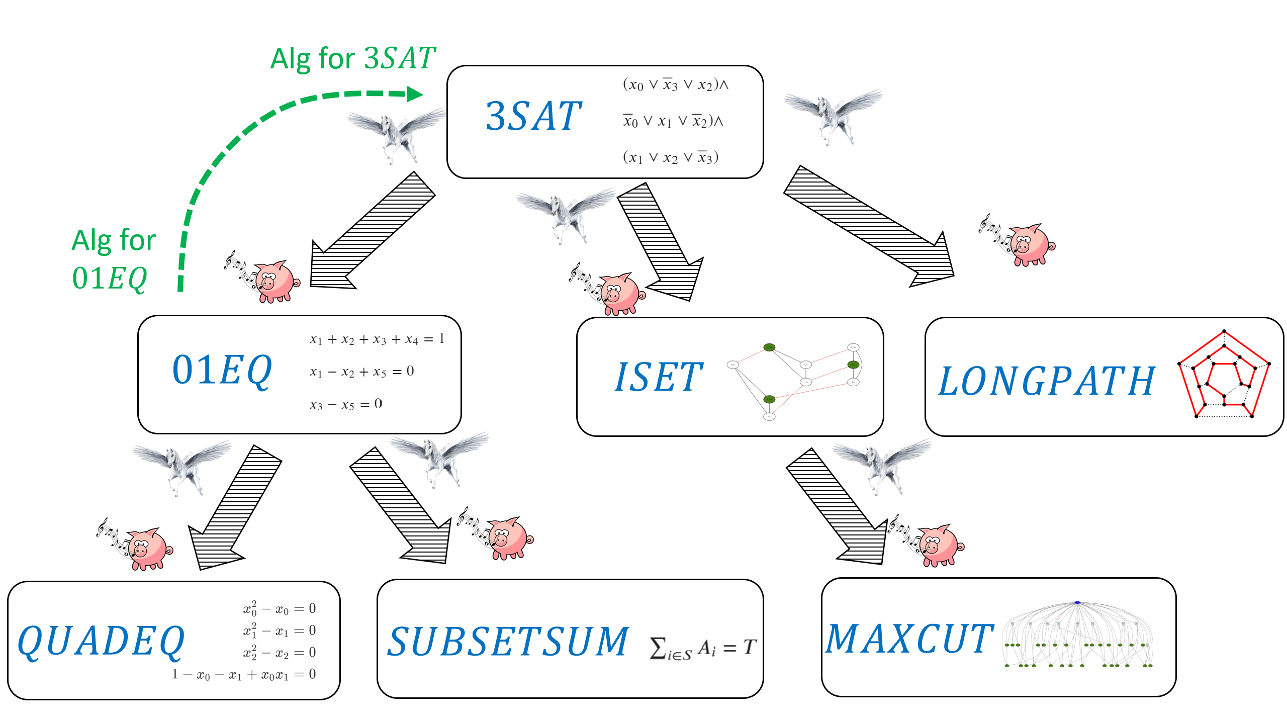
In this chapter we will see that for each one of the problems of finding a longest path in a graph, solving quadratic equations, and finding the maximum cut, if there exists a polynomial-time algorithm for this problem then there exists a polynomial-time algorithm for the 3SAT problem as well. In other words, we will reduce the task of solving 3SAT to each one of the above tasks. Another way to interpret these results is that if there does not exist a polynomial-time algorithm for 3SAT then there does not exist a polynomial-time algorithm for these other problems as well. In Chapter 15 we will see evidence (though no proof!) that all of the above problems do not have polynomial-time algorithms and hence are inherently intractable.
Formal definitions of problems
For reasons of technical convenience rather than anything substantial, we concern ourselves with decision problems (i.e., Yes/No questions) or in other words Boolean (i.e., one-bit output) functions. We model the problems above as functions mapping \(\{0,1\}^*\) to \(\{0,1\}\) in the following way:
3SAT. The 3SAT problem can be phrased as the function \(3\ensuremath{\mathit{SAT}}:\{0,1\}^* \rightarrow \{0,1\}\) that takes as input a 3CNF formula \(\varphi\) (i.e., a formula of the form \(C_0 \wedge \cdots \wedge C_{m-1}\) where each \(C_i\) is the OR of three variables or their negation) and maps \(\varphi\) to \(1\) if there exists some assignment to the variables of \(\varphi\) that causes it to evalute to true, and to \(0\) otherwise. For example
since the assignment \(x = 1101\) satisfies the input formula. In the above we assume some representation of formulas as strings, and define the function to output \(0\) if its input is not a valid representation; we use the same convention for all the other functions below.
Quadratic equations. The quadratic equations problem corresponds to the function \(\ensuremath{\mathit{QUADEQ}}:\{0,1\}^* \rightarrow \{0,1\}\) that maps a set of quadratic equations \(E\) to \(1\) if there is an assignment \(x\) that satisfies all equations, and to \(0\) otherwise.
Longest path. The longest path problem corresponds to the function \(\ensuremath{\mathit{LONGPATH}}:\{0,1\}^* \rightarrow \{0,1\}\) that maps a graph \(G\) and a number \(k\) to \(1\) if there is a simple path in \(G\) of length at least \(k\), and maps \((G,k)\) to \(0\) otherwise. The longest path problem is a generalization of the well-known Hamiltonian Path Problem of determining whether a path of length \(n\) exists in a given \(n\) vertex graph.
Maximum cut. The maximum cut problem corresponds to the function \(\ensuremath{\mathit{MAXCUT}}:\{0,1\}^* \rightarrow \{0,1\}\) that maps a graph \(G\) and a number \(k\) to \(1\) if there is a cut in \(G\) that cuts at least \(k\) edges, and maps \((G,k)\) to \(0\) otherwise.
All of the problems above are in \(\mathbf{EXP}\) but it is not known whether or not they are in \(\mathbf{P}\). However, we will see in this chapter that if either \(\ensuremath{\mathit{QUADEQ}}\) , \(\ensuremath{\mathit{LONGPATH}}\) or \(\ensuremath{\mathit{MAXCUT}}\) are in \(\mathbf{P}\), then so is \(3\ensuremath{\mathit{SAT}}\).
Polynomial-time reductions
Suppose that \(F,G:\{0,1\}^* \rightarrow \{0,1\}\) are two Boolean functions. A polynomial-time reduction (or sometimes just “reduction” for short) from \(F\) to \(G\) is a way to show that \(F\) is “no harder” than \(G\), in the sense that a polynomial-time algorithm for \(G\) implies a polynomial-time algorithm for \(F\).
Let \(F,G:\{0,1\}^* \rightarrow \{0,1\}\). We say that \(F\) reduces to \(G\), denoted by \(F \leq_p G\) if there is a polynomial-time computable \(R:\{0,1\}^* \rightarrow \{0,1\}^*\) such that for every \(x\in \{0,1\}^*\), We say that \(F\) and \(G\) have equivalent complexity if \(F \leq_p G\) and \(G \leq_p F\).
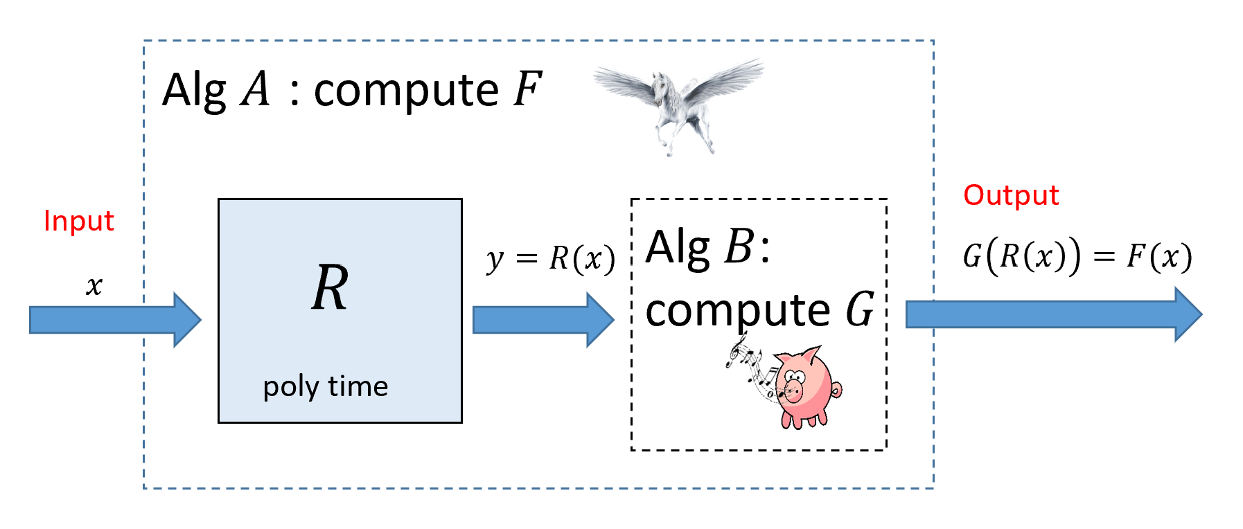
The following exercise justifies our intuition that \(F \leq_p G\) signifies that “\(F\) is no harder than \(G\)”.
Prove that if \(F \leq_p G\) and \(G \in \mathbf{P}\) then \(F\in \mathbf{P}\).
As usual, solving this exercise on your own is an excellent way to make sure you understand Definition 14.1.
Suppose there is an algorithm \(B\) that computes \(G\) in time \(p(n)\) where \(n\) is its input size. Then, Equation 14.1 directly gives an algorithm \(A\) to compute \(F\) (see Figure 14.2). Indeed, on input \(x\in \{0,1\}^*\), Algorithm \(A\) will run the polynomial-time reduction \(R\) to obtain \(y=R(x)\) and then return \(B(y)\). By Equation 14.1, \(G(R(x)) = F(x)\) and hence Algorithm \(A\) will indeed compute \(F\).
We now show that \(A\) runs in polynomial time. By assumption, \(R\) can be computed in time \(q(n)\) for some polynomial \(q\). In particular, this means that \(|y| \leq q(|x|)\) (as just writing down \(y\) takes \(|y|\) steps). Computing \(B(y)\) will take at most \(p(|y|) \leq p(q(|x|))\) steps. Thus the total running time of \(A\) on inputs of length \(n\) is at most the time to compute \(y\), which is bounded by \(q(n)\), and the time to compute \(B(y)\), which is bounded by \(p(q(n))\), and since the composition of two polynomials is a polynomial, \(A\) runs in polynomial time.
A reduction \(F \leq_p G\) shows that \(F\) is “no harder than \(G\)” or equivalently that \(G\) is “no easier than \(F\)”.
Whistling pigs and flying horses
A reduction from \(F\) to \(G\) can be used for two purposes:
If we already know an algorithm for \(G\) and \(F \leq_p G\) then we can use the reduction to obtain an algorithm for \(F\). This is a widely used tool in algorithm design. For example in Section 12.1.4 we saw how the Min-Cut Max-Flow theorem allows to reduce the task of computing a minimum cut in a graph to the task of computing a maximum flow in it.
If we have proven (or have evidence) that there exists no polynomial-time algorithm for \(F\) and \(F \leq_p G\) then the existence of this reduction allows us to conclude that there exists no polynomial-time algorithm for \(G\). This is the “if pigs could whistle then horses could fly” interpretation we’ve seen in Section 9.4. We show that if there was an hypothetical efficient algorithm for \(G\) (a “whistling pig”) then since \(F \leq_p G\) then there would be an efficient algorithm for \(F\) (a “flying horse”). In this book we often use reductions for this second purpose, although the lines between the two is sometimes blurry (see the bibliographical notes in Section 14.10).
The most crucial difference between the notion in Definition 14.1 and the reductions we saw in the context of uncomputability (e.g., in Section 9.4) is that for relating time complexity of problems, we need the reduction to be computable in polynomial time, as opposed to merely computable. Definition 14.1 also restricts reductions to have a very specific format. That is, to show that \(F \leq_p G\), rather than allowing a general algorithm for \(F\) that uses a “magic box” that computes \(G\), we only allow an algorithm that computes \(F(x)\) by outputting \(G(R(x))\). This restricted form is convenient for us, but people have defined and used more general reductions as well (see Section 14.10).
In this chapter we use reductions to relate the computational complexity of the problems mentioned above: 3SAT, Quadratic Equations, Maximum Cut, and Longest Path, as well as a few others. We will reduce 3SAT to the latter problems, demonstrating that solving any one of them efficiently will result in an efficient algorithm for 3SAT. In Chapter 15 we show the other direction: reducing each one of these problems to 3SAT in one fell swoop.
Transitivity of reductions. Since we think of \(F \leq_p G\) as saying that (as far as polynomial-time computation is concerned) \(F\) is “easier or equal in difficulty to” \(G\), we would expect that if \(F \leq_p G\) and \(G \leq_p H\), then it would hold that \(F \leq_p H\). Indeed this is the case:
For every \(F,G,H :\{0,1\}^* \rightarrow \{0,1\}\), if \(F \leq_p G\) and \(G \leq_p H\) then \(F \leq_p H\).
If \(F \leq_p G\) and \(G \leq_p H\) then there exist polynomial-time computable functions \(R_1\) and \(R_2\) mapping \(\{0,1\}^*\) to \(\{0,1\}^*\) such that for every \(x\in \{0,1\}^*\), \(F(x) = G(R_1(x))\) and for every \(y\in \{0,1\}^*\), \(G(y) = H(R_2(y))\). Combining these two equalities, we see that for every \(x\in \{0,1\}^*\), \(F(x) = H(R_2(R_1(x)))\) and so to show that \(F \leq_p H\), it is sufficient to show that the map \(x \mapsto R_2(R_1(x))\) is computable in polynomial time. But if there are some constants \(c,d\) such that \(R_1(x)\) is computable in time \(|x|^c\) and \(R_2(y)\) is computable in time \(|y|^d\) then \(R_2(R_1(x))\) is computable in time \((|x|^c)^d = |x|^{cd}\) which is polynomial.
Reducing 3SAT to zero one and quadratic equations
We now show our first example of a reduction. The Zero-One Linear Equations problem corresponds to the function \(01\ensuremath{\mathit{EQ}}:\{0,1\}^* \rightarrow \{0,1\}\) whose input is a collection \(E\) of linear equations in variables \(x_0,\ldots,x_{n-1}\), and the output is \(1\) iff there is an assignment \(x\in \{0,1\}^n\) of \(0/1\) values to the variables that satisfies all the equations. For example, if the input \(E\) is a string encoding the set of equations
then \(01\ensuremath{\mathit{EQ}}(E)=1\) since the assignment \(x = 011\) satisfies all three equations. We specifically restrict attention to linear equations in variables \(x_0,\ldots, x_{n-1}\) in which every equation has the form \(\sum_{i \in S} x_i = b\) where \(S \subseteq [n]\) and \(b\in \N\).1
If we asked the question of whether there is a solution \(x \in \R^n\) of real numbers to \(E\), then this can be solved using the famous Gaussian elimination algorithm in polynomial time. However, there is no known efficient algorithm to solve \(01\ensuremath{\mathit{EQ}}\). Indeed, such an algorithm would imply an algorithm for \(3\ensuremath{\mathit{SAT}}\) as shown by the following theorem:
\(3\ensuremath{\mathit{SAT}} \leq_p 01\ensuremath{\mathit{EQ}}\)
A constraint \(x_2 \vee \overline{x}_5 \vee x_7\) can be written as \(x_2 + (1-x_5) + x_7 \geq 1\). This is a linear inequality but since the sum on the left-hand side is at most three, we can also turn it into an equality by adding two new variables \(y,z\) and writing it as \(x_2 + (1-x_5) + x_7 + y + z =3\). (We will use fresh variables \(y,z\) for every constraint.) Finally, for every variable \(x_i\) we can add a variable \(x'_i\) corresponding to its negation by adding the equation \(x_i + x'_i = 1\), hence mapping the original constraint \(x_2 \vee \overline{x}_5 \vee x_7\) to \(x_2 + x'_5 + x_7 +y + z = 3\). The main takeaway technique from this reduction is the idea of adding auxiliary variables to replace an equation such as \(x_1+x_2 +x_3 \geq 1\) that is not quite in the form we want with the equivalent (for \(0/1\) valued variables) equation \(x_1+x_2+x_3+u+v=3\) which is in the form we want.

To prove the theorem we need to:
Describe an algorithm \(R\) for mapping an input \(\varphi\) for \(3\ensuremath{\mathit{SAT}}\) into an input \(E\) for \(01\ensuremath{\mathit{EQ}}\).
Prove that the algorithm runs in polynomial time.
Prove that \(01\ensuremath{\mathit{EQ}}(R(\varphi)) =3\ensuremath{\mathit{SAT}}(\varphi)\) for every 3CNF formula \(\varphi\).
We now proceed to do just that. Since this is our first reduction, we will spell out this proof in detail. However it straightforwardly follows the proof idea.
Algorithm 14.3 3SAT to 01EQ reduction
Input: 3CNF formula \(\varphi\) with \(n\) variables \(x_0,\ldots,x_{n-1}\) and \(m\) clauses.
Output: Set \(E\) of linear equations over \(0/1\) such that \(3SAT(\varphi)=1\) iff \(01EQ(E)=1\).
Let \(E\)'s variables be \(x_0,\ldots,x_{n-1}\), \(x'_0,\ldots,x'_{n-1}\), \(y_0,\ldots,y_{m-1}\), \(z_0,\ldots,z_{m-1}\).
for{\(i \in [n]\)}
add to \(E\) the equation \(x_i + x'_i = 1\)
endfor
for{\(j\in [m]\)}
Let \(j\)-th clause be \(w_0 \vee w_1 \vee w_2\) where \(w_0,w_1,w_2\) are literals.
for{\(a\in[3]\)}
if{\(w_a\) is variable \(x_i\)}
set \(t_a \leftarrow x_i\)
endif
if{\(w_a\) is negation \(\neg x_i\)}
set \(t_a \leftarrow x'_i\)
endif
endfor
Add to \(E\) the equation \(t_0 + t_1 + t_2 + y_j + z_j = 3\).
endfor
return \(E\)
The reduction is described in Algorithm 14.3, see also Figure 14.3. If the input formula has \(n\) variables and \(m\) clauses, Algorithm 14.3 creates a set \(E\) of \(n+m\) equations over \(2n+2m\) variables. Algorithm 14.3 makes an initial loop of \(n\) steps (each taking constant time) and then another loop of \(m\) steps (each taking constant time) to create the equations, and hence it runs in polynomial time.
Let \(R\) be the function computed by Algorithm 14.3. The heart of the proof is to show that for every 3CNF \(\varphi\), \(01\ensuremath{\mathit{EQ}}(R(\varphi)) = 3\ensuremath{\mathit{SAT}}(\varphi)\). We split the proof into two parts. The first part, traditionally known as the completeness property, is to show that if \(3\ensuremath{\mathit{SAT}}(\varphi)=1\) then \(01\ensuremath{\mathit{EQ}}(R(\varphi))=1\). The second part, traditionally known as the soundness property, is to show that if \(01\ensuremath{\mathit{EQ}}(R(\varphi))=1\) then \(3\ensuremath{\mathit{SAT}}(\varphi)=1\). (The names “completeness” and “soundness” derive viewing a solution to \(R(\varphi)\) as a “proof” that \(\varphi\) is satisfiable, in which case these conditions corresponds to completeness and soundness as defined in Section 11.1.1. However, if you find the names confusing you can simply think of completeness as the “\(1\)-instance maps to \(1\)-instance” property and soundness as the “\(0\)-instance maps to \(0\)-instance” property.)
We complete the proof by showing both parts:
Completeness: Suppose that \(3\ensuremath{\mathit{SAT}}(\varphi)=1\), which means that there is an assignment \(x\in \{0,1\}^n\) that satisfies \(\varphi\). If we use the assignment \(x_0,\ldots,x_{n-1}\) and \(1-x_0,\ldots, 1-x_{n-1}\) for the first \(2n\) variables of \(E=R(\varphi)\) then we will satisfy all equations of the form \(x_i + x'_i =1\). Moreover, for every \(j\in [m]\), if \(t_0 + t_1 + t_2 + y_j + z_j = 3 (*)\) is the equation arising from the \(j\)th clause of \(\varphi\) (with \(t_0,t_1,t_2\) being variables of the form \(x_i\) or \(x'_i\) depending on the literals of the clause) then our assignment to the first \(2n\) variables ensures that \(t_0+t_1+t_2 \geq 1\) (since \(x\) satisfied \(\varphi\)) and hence we can assign values to \(y_j\) and \(z_j\) that will ensure that the equation \((*)\) is satisfied. Hence in this case \(E = R(\varphi)\) is satisfied, meaning that \(01\ensuremath{\mathit{EQ}}(R(\varphi))=1\).
Soundness: Suppose that \(01\ensuremath{\mathit{EQ}}(R(\varphi))=1\), which means that the set of equations \(E=R(\varphi)\) has a satisfying assignment \(x_0,\ldots,x_{n-1}\), \(x'_0,\ldots,x'_{n-1}\), \(y_0,\ldots,y_{m-1}\), \(z_0,\ldots,z_{m-1}\). Then, since the equations contain the condition \(x_i + x'_i = 1\), for every \(i \in [n]\), \(x'_i\) is the negation of \(x_i\), and morover, for every \(j\in [m]\), if \(C\) has the form \(w_0 \vee w_1 \vee w_2\) and is the \(j\)-th clause of \(\varphi\), then the corresponding assignment \(x\) will ensure that \(w_0 + w_1 + w_2 \geq 1\), implying that \(C\) is satisfied. Hence in this case \(3\ensuremath{\mathit{SAT}}(\varphi)=1\).
Quadratic equations
Now that we reduced \(3\ensuremath{\mathit{SAT}}\) to \(01\ensuremath{\mathit{EQ}}\), we can use this to reduce \(3\ensuremath{\mathit{SAT}}\) to the quadratic equations problem. This is the function \(\ensuremath{\mathit{QUADEQ}}\) in which the input is a list of \(n\)-variate polynomials \(p_0,\ldots,p_{m-1}:\R^n \rightarrow \R\) that are all of degree at most two (i.e., they are quadratic) and with integer coefficients. (The latter condition is for convenience and can be achieved by scaling.) We define \(\ensuremath{\mathit{QUADEQ}}(p_0,\ldots,p_{m-1})\) to equal \(1\) if and only if there is a solution \(x\in \R^n\) to the equations \(p_0(x)=0\), \(p_1(x)=0\), \(\ldots\), \(p_{m-1}(x)=0\).
For example, the following is a set of quadratic equations over the variables \(x_0,x_1,x_2\):
Using the transitivity of reductions (Solved Exercise 14.2), it is enough to show that \(01\ensuremath{\mathit{EQ}} \leq_p \ensuremath{\mathit{QUADEQ}}\), but this follows since we can phrase the equation \(x_i \in \{0,1\}\) as the quadratic constraint \(x_i^2 - x_i = 0\). The takeaway technique of this reduction is that we can use non-linearity to force continuous variables (e.g., variables taking values in \(\R\)) to be discrete (e.g., take values in \(\{0,1\}\)).
By Theorem 14.2 and Solved Exercise 14.2, it is sufficient to prove that \(01\ensuremath{\mathit{EQ}} \leq_p \ensuremath{\mathit{QUADEQ}}\). Let \(E\) be an instance of \(01\ensuremath{\mathit{EQ}}\) with variables \(x_0,\ldots,x_{n-1}\). We map \(E\) to the set of quadratic equations \(E'\) that is obtained by taking the linear equations in \(E\) and adding to them the \(n\) quadratic equations \(x_i^2 - x_i = 0\) for all \(i\in [n]\). (See Algorithm 14.5.) The map \(E \mapsto E'\) can be computed in polynomial time. We claim that \(01\ensuremath{\mathit{EQ}}(E)=1\) if and only if \(\ensuremath{\mathit{QUADEQ}}(E')=1\). Indeed, the only difference between the two instances is that:
In the \(01\ensuremath{\mathit{EQ}}\) instance \(E\), the equations are over variables \(x_0,\ldots,x_{n-1}\) in \(\{0,1\}\).
In the \(\ensuremath{\mathit{QUADEQ}}\) instance \(E'\), the equations are over variables \(x_0,\ldots,x_{n-1} \in \R\) but we have the extra constraints \(x_i^2 - x_i = 0\) for all \(i\in [n]\).
Since for every \(a\in \R\), \(a^2 - a = 0\) if and only if \(a \in \{0,1\}\), the two sets of equations are equivalent and \(01\ensuremath{\mathit{EQ}}(E)=\ensuremath{\mathit{QUADEQ}}(E')\) which is what we wanted to prove.
Algorithm 14.5 01EQ to QUADEQ reduction
Input: Set \(E\) of linear equations over \(n\) variables \(x_0,\ldots,x_{n-1}\).
Output: Set \(E'\) of quadratic equations over \(m\) variables \(w_0,\ldots,w_{m-1}\) such that there is an \(0/1\) assignment \(x\in \{0,1\}^n\)
satisfying the equations of \(E\) iff there is an assignment \(w \in \R^m\) satisfying the equations of \(E'\).
That is, \(01EQ(E) = QUADEQ(E')\).
Let \(m \leftarrow n\).
Variables of \(E'\) are set to be same variable \(x_0,\ldots, x_{n-1}\) as \(E\).
for{every equation \(e\in E\)}
Add \(e\) to \(E'\)
endfor
for{\(i\in [n]\)}
Add to \(E'\) the equation \(x_i^2 - x_i = 0\).
endfor
return \(E'\)
The subset sum problem
As another consequence of the reduction of \(3\ensuremath{\mathit{SAT}}\) to \(01\ensuremath{\mathit{EQ}}\), we can also show that \(3\ensuremath{\mathit{SAT}}\) (through \(01\ensuremath{\mathit{EQ}}\)) reduces to the subset sum problem (also known as the knapsack problem). In the subset sum problem, we are given a list of integers \(x_0,\ldots,x_{n-1} \in \mathbb{Z}\) and an integer \(T\in\mathbb{Z}\). We need to determine whether or not there exists some set of the integers that sums up to \(T\). That is, for \(x_0,\ldots,x_{n-1},T \in \mathbb{Z}\), \(\ensuremath{\mathit{SSUM}}(x_0,\ldots,x_{n-1},T)=1\) if and only if there exists \(S\subseteq [n]\) such that \(\sum_{i\in S} x_i = T\). Note that the input length for the subset sum problem is the length of string needed to encode all the numbers, which will be approximately \(\lceil \log T \rceil + \sum_{i=0}^n \lceil \log x_i \rceil\), since encoding an integer \(x\) using the binary representation requires \(\lceil \log x \rceil\) bits.
We reduce from \(01\ensuremath{\mathit{EQ}}\). The intuition is the following. Consider an instance \(E\) of \(01\ensuremath{\mathit{EQ}}\) with \(n\) variables \(x_0,\ldots,x_{n-1}\) and \(m\) equations \(e_0,\ldots,e_{m-1}\). Recall that each equation \(e_\ell\) in \(E\) has the form \(x_i + x_j + x_k = b\) (potentially with more or less than three variables summed up on the left-hand side of the equation). For every variable \(x_i\), we can define a vector \(v^i \in \{0,1\}^m\) where \(v^i_t=1\) if the variable \(x_i\) appears in the equation \(e_t\) and \(v^i_t=0\) otherwise. Then there is a solution to the set of equations if and only if there is some set \(S\subseteq [n]\) (corresponding to the \(i\)’s such that \(x_i=1\)) such that \(\sum_{i\in S} v^i = \vec{b}\) where \(\vec{b} \in \mathbb{Z}^m\) is the vector of right hand sides of the equations (i.e., \(\vec{b}_t\) is the value \(b_t\) on the righthand side of the \(t\)-th equation). Now if we could interpret the vectors \(v^0,\ldots,v^{n-1}\) and \(\vec{b}\) as numbers then we could think of this as a subset sum instance. The key insight is that we can in fact think of vectors as numbers by thinking of the \(j\)-th coordinate of the vector \(v\) as the \(j\)-th digit. Since the vectors are in \(\{0,1\}^m\), the natural choice is to use the binary basis, but this turns out to cause issues with “carries” when we add them up. Hence we use a larger basis \(B\), see proof below.
For a given set of \(01\ensuremath{\mathit{EQ}}\) on \(n\) variables, we note that the right hand side can never be larger than \(n\) (since the sum of at most \(n\) variables in \(\{0,1\}\) is at most \(n\)). More concretely, if the instance has such an equation then we can know for sure that the answer is \(0\) (and in the context of a reduction map it into some trivial instance of subset sum that doesn’t have a solution such as \(x_0=x_1=1\) and \(T=3\)).
Our reduction is described in Algorithm 14.7. On input an instance \(E = \{ e_t \}_{t=1}^m\) of \(01\ensuremath{\mathit{EQ}}\) over \(n\) variables \(x_0,\ldots,x_{n-1}\), we output an \(\ensuremath{\mathit{SSUM}}\) instance \(y_0,\ldots,y_{n-1},T\) computed as follows:
\(y_i = \sum_{t=0}^{m-1} B^t v^i_t\) where \(v^i_t\) equals \(1\) if the variable \(x_i\) appears in the equation \(e_t\) and equals \(0\) otherwise. The number \(B\) is set to be \(2n\) (any numb er larger than \(n\) would work.)
\(T = \sum_{t=0}^{m-1} B^t b_t\) where \(b_t\) is the integer on the right-hand side of the equation \(e_t\).
In other words, \(y_0,\ldots,y_{n-1}\) and \(T\) are the integers such that, written in the \(B\)-ary basis, the \(t\)-th digit of \(y_i\) is \(1\) iff \(x_i\) appears in \(x_t\), and the \(t\)-th digit of \(T\) is the right-hand side of \(e_t\).
The following claim will imply the correctness of the reduction:
Claim: For every \(x\in \{0,1\}^n\), if \(S = \{ i | x_i = 1 \}\) then \(x\) satisfies the equations of \(E\) if and only if \(\sum_{i\in S} y_i = T\).
Proof: Key to the proof is the following simple property of gradeschool addition: when adding at most \(n\) numbers in the \(B\)-ary basis, if all the numbers have all their digits either \(0\) or \(1\), and \(B>n\), then for every \(t\), the \(t\)-th digit of the sum is the sum of the \(t\)-th digits of the numbers. This is a simple consequence of the fact that there is no “carry” in the addition. Since in our case the numbers \(y_0,\ldots,y_n\) satisfy this property in the \(B\)-ary basis, and \(B>n\), we get that for every \(S \subseteq [n]\) and every digit \(t\), the \(t\)-th digit of the sum \(\sum_{i\in S}y_i\) is simply the sum of the \(t\)-th digit, which would correspond to the sum over \(x_i\) for all \(x_i\)’s that participate in the \(t\)-th equation. This sum would equal the \(t\)-th digit of \(T\) if and only if that equation is satisfied.
The claim shows that \(01\ensuremath{\mathit{EQ}}(E) = \ensuremath{\mathit{SSUM}}(y_0,\ldots,y_{n-1},T)\) which is what we needed to prove.
Algorithm 14.7 01EQ to SSUM reduction
Input: Set \(E = \{ e_t \}_{t\in [m]}\) of \(m\) linear equations over \(n\) variables \(x_0,\ldots,x_{n-1}\).
Output: Numbers \(y_0,\ldots,y_{n-1},T \in \mathbb{Z}\) such that there is an \(0/1\) assignment \(x\in \{0,1\}^n\) satisfying the equations of \(E\) iff there is \(S \subseteq [n]\) such that \(\sum_{i\in S}y_i = T\).
for{every equation \(e_t\in E\)}
Let \(A \subseteq [n]\) and \(b\in \mathbb{Z}\) be such that \(e_t\) has the form \(\sum_{i\in A} x_i = b\)
Let \(v_i^t \leftarrow 1\) if \(i\in A\) and \(v_i^t \leftarrow 0\) otherwise.
Let \(b_t \leftarrow b\).
endfor
Set \(B \leftarrow 2n\)
for{\(i\in [n]\)}
Let \(y_i \leftarrow \sum_{t=1}^m B^t v_i^t\).
endfor
Let \(T \leftarrow \sum_{t=1}^T B^t b_t\)
return \(y_0,\ldots,y_{n-1},T\)
The independent set problem
For a graph \(G=(V,E)\), an independent set (also known as a stable set) is a subset \(S \subseteq V\) such that there are no edges with both endpoints in \(S\) (in other words, \(E(S,S)=\emptyset\)). Every “singleton” (set consisting of a single vertex) is trivially an independent set, but finding larger independent sets can be challenging. The maximum independent set problem (henceforth simply “independent set”) is the task of finding the largest independent set in the graph. The independent set problem is naturally related to scheduling problems: if we put an edge between two conflicting tasks, then an independent set corresponds to a set of tasks that can all be scheduled together without conflicts. The independent set problem has been studied in a variety of settings, including for example in the case of algorithms for finding structure in protein-protein interaction graphs.
As mentioned in Section 14.1, we think of the independent set problem as the function \(\ensuremath{\mathit{ISET}}:\{0,1\}^* \rightarrow \{0,1\}\) that on input a graph \(G\) and a number \(k\) outputs \(1\) if and only if the graph \(G\) contains an independent set of size at least \(k\). We now reduce 3SAT to Independent set.
\(3\ensuremath{\mathit{SAT}} \leq_p \ensuremath{\mathit{ISET}}\).
The idea is that finding a satisfying assignment to a 3SAT formula corresponds to satisfying many local constraints without creating any conflicts. One can think of “\(x_{17}=0\)” and “\(x_{17}=1\)” as two conflicting events, and of the constraints \(x_{17} \vee \overline{x}_5 \vee x_9\) as creating a conflict between the events “\(x_{17}=0\)”, “\(x_5=1\)” and “\(x_9=0\)”, saying that these three cannot simultaneously co-occur. Using these ideas, we can we can think of solving a 3SAT problem as trying to schedule non-conflicting events, though the devil is, as usual, in the details. The takeaway technique here is to map each clause of the original formula into a gadget which is a small subgraph (or more generally “subinstance”) satisfying some convenient properties. We will see these “gadgets” used time and again in the construction of polynomial-time reductions.

Algorithm 14.9 3SAT to IS reduction
Input: \(3SAT\) formula \(\varphi\) with \(n\) variables and \(m\) clauses.
Output: Graph \(G=(V,E)\) and number \(k\), such that \(G\) has an independent set of size \(k\) iff \(\varphi\) has a satisfying assignment.
That is, \(3SAT(\varphi) = ISET(G,k)\),
Initialize \(V \leftarrow \emptyset, E \leftarrow \emptyset\)
for {every clause \(C = y \vee y' \vee y''\) of \(\varphi\)}
Add three vertices \((C,y),(C,y'),(C,y'')\) to \(V\)
Add edges \(\{ (C,y), (C,y') \}\), \(\{(C,y'),(C,y'') \}\), \(\{ (C,y''), (C,y) \}\) to \(E\).
endfor
for {every distinct clauses \(C,C'\) in \(\varphi\)}
for {every \(i\in [n]\)}
if{\(C\) contains literal \(x_i\) and \(C'\) contains literal \(\overline{x}_i\)}
Add edge \(\{ (C,x_i), (C',\overline{x}_i) \}\) to \(E\)
endif
endfor
endfor
return \((G=(V,E), m)\)
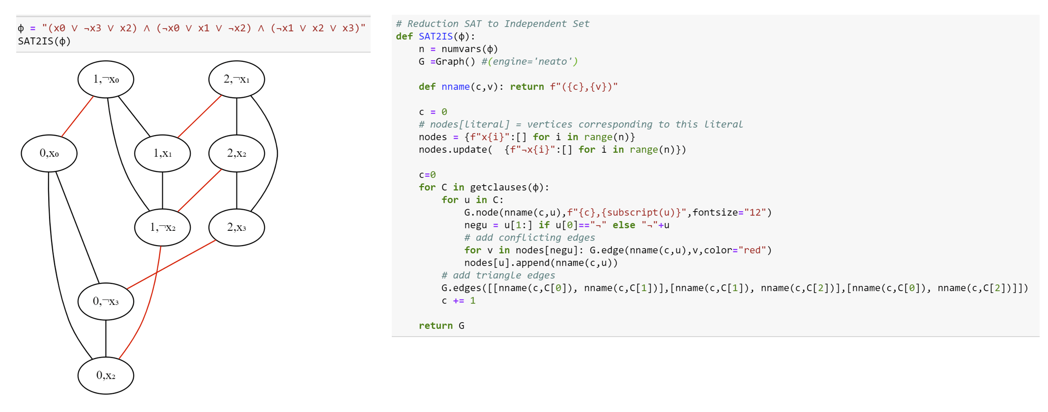
Given a 3SAT formula \(\varphi\) on \(n\) variables and with \(m\) clauses, we will create a graph \(G\) with \(3m\) vertices as follows. (See Algorithm 14.9, see also Figure 14.4 for an example and Figure 14.5 for Python code.)
A clause \(C\) in \(\varphi\) has the form \(C = y \vee y' \vee y''\) where \(y,y',y''\) are literals (variables or their negation). For each such clause \(C\), we will add three vertices to \(G\), and label them \((C,y)\), \((C,y')\), and \((C,y'')\) respectively. We will also add the three edges between all pairs of these vertices, so they form a triangle. Since there are \(m\) clauses in \(\varphi\), the graph \(G\) will have \(3m\) vertices.
In addition to the above edges, we also add an edge between every pair of vertices of the form \((C,y)\) and \((C',y')\) where \(y\) and \(y'\) are conflicting literals. That is, we add an edge between \((C,y)\) and \((C',y')\) if there is an \(i\) such that \(y=x_i\) and \(y' = \overline{x}_i\) or vice versa.
The algorithm constructing \(G\) based on \(\varphi\) takes polynomial time since it involves two loops, the first taking \(O(m)\) steps and the second taking \(O(m^2 n)\) steps (see Algorithm 14.9). Hence to prove the theorem we need to show that \(\varphi\) is satisfiable if and only if \(G\) contains an independent set of \(m\) vertices. We now show both directions of this equivalence:
Part 1: Completeness. The “completeness” direction is to show that if \(\varphi\) has a satisfying assignment \(x^*\), then \(G\) has an independent set \(S^*\) of \(m\) vertices. Let us now show this.
Indeed, suppose that \(\varphi\) has a satisfying assignment \(x^* \in \{0,1\}^n\). Then for every clause \(C = y \vee y' \vee y''\) of \(\varphi\), one of the literals \(y,y',y''\) must evaluate to true under the assignment \(x^*\) (as otherwise it would not satisfy \(\varphi\)). We let \(S\) be a set of \(m\) vertices that is obtained by choosing for every clause \(C\) one vertex of the form \((C,y)\) such that \(y\) evaluates to true under \(x^*\). (If there is more than one such vertex for the same \(C\), we arbitrarily choose one of them.)
We claim that \(S\) is an independent set. Indeed, suppose otherwise that there was a pair of vertices \((C,y)\) and \((C',y')\) in \(S\) that have an edge between them. Since we picked one vertex out of each triangle corresponding to a clause, it must be that \(C \neq C'\). Hence the only way that there is an edge between \((C,y)\) and \((C',y')\) is if \(y\) and \(y'\) are conflicting literals (i.e. \(y=x_i\) and \(y'=\overline{x}_i\) for some \(i\)). But then they can’t both evaluate to true under the assignment \(x^*\), which contradicts the way we constructed the set \(S\). This completes the proof of the completeness condition.
Part 2: Soundness. The “soundness” direction is to show that if \(G\) has an independent set \(S^*\) of \(m\) vertices, then \(\varphi\) has a satisfying assignment \(x^* \in \{0,1\}^n\). Let us now show this.
Indeed, suppose that \(G\) has an independent set \(S^*\) with \(m\) vertices. We will define an assignment \(x^* \in \{0,1\}^n\) for the variables of \(\varphi\) as follows. For every \(i\in [n]\), we set \(x^*_i\) according to the following rules:
If \(S^*\) contains a vertex of the form \((C,x_i)\) then we set \(x^*_i=1\).
If \(S^*\) contains a vertex of the form \((C,\overline{x_i})\) then we set \(x^*_i=0\).
If \(S^*\) does not contain a vertex of either of these forms, then it does not matter which value we give to \(x^*_i\), but for concreteness we’ll set \(x^*_i=0\).
The first observation is that \(x^*\) is indeed well defined, in the sense that the rules above do not conflict with one another, and ask to set \(x^*_i\) to be both \(0\) and \(1\). This follows from the fact that \(S^*\) is an independent set and hence if it contains a vertex of the form \((C,x_i)\) then it cannot contain a vertex of the form \((C',\overline{x_i})\).
We now claim that \(x^*\) is a satisfying assignment for \(\varphi\). Indeed, since \(S^*\) is an independent set, it cannot have more than one vertex inside each one of the \(m\) triangles \((C,y),(C,y'),(C,y'')\) corresponding to a clause of \(\varphi\). Hence since \(|S^*|=m\), it must have exactly one vertex in each such triangle. For every clause \(C\) of \(\varphi\), if \((C,y)\) is the vertex in \(S^*\) in the triangle corresponding to \(C\), then by the way we defined \(x^*\), the literal \(y\) must evaluate to true, which means that \(x^*\) satisfies this clause. Therefore \(x^*\) satisfies all clauses of \(\varphi\), which is the definition of a satisfying assignment.
This completes the proof of Theorem 14.8
Some exercises and anatomy of a reduction.
Reductions can be confusing and working out exercises is a great way to gain more comfort with them. Here is one such example. As usual, I recommend you try it out yourself before looking at the solution.
A vertex cover in a graph \(G=(V,E)\) is a subset \(S \subseteq V\) of vertices such that every edge touches at least one vertex of \(S\) (see Figure 14.6). The vertex cover problem is the task to determine, given a graph \(G\) and a number \(k\), whether there exists a vertex cover in the graph with at most \(k\) vertices. Formally, this is the function \(\ensuremath{\mathit{VC}}:\{0,1\}^* \rightarrow \{0,1\}\) such that for every \(G=(V,E)\) and \(k\in \N\), \(\ensuremath{\mathit{VC}}(G,k)=1\) if and only if there exists a vertex cover \(S \subseteq V\) such that \(|S| \leq k\).
Prove that \(3\ensuremath{\mathit{SAT}} \leq_p \ensuremath{\mathit{VC}}\).
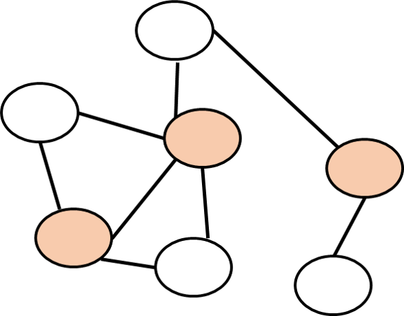
The key observation is that if \(S \subseteq V\) is a vertex cover that touches all vertices, then there is no edge \(e\) such that both \(e\)’s endpoints are in the set \(\overline{S} = V \setminus S\), and vice versa. In other words, \(S\) is a vertex cover if and only if \(\overline{S}\) is an independent set. Since the size of \(\overline{S}\) is \(|V|-|S|\), we see that the polynomial-time map \(R(G,k)=(G,n-k)\) (where \(n\) is the number of vertices of \(G\)) satisfies that \(\ensuremath{\mathit{VC}}(R(G,k))= \ensuremath{\mathit{ISET}}(G,k)\) which means that it is a reduction from independent set to vertex cover.
The maximum clique problem corresponds to the function \(\ensuremath{\mathit{CLIQUE}}:\{0,1\}^* \rightarrow \{0,1\}\) such that for a graph \(G\) and a number \(k\), \(\ensuremath{\mathit{CLIQUE}}(G,k)=1\) iff there is a subset \(S\) of \(k\) vertices such that for every distinct \(u,v \in S\), the edge \(u,v\) is in \(G\). Such a set is known as a clique.
Prove that \(\ensuremath{\mathit{CLIQUE}} \leq_p \ensuremath{\mathit{ISET}}\) and \(\ensuremath{\mathit{ISET}} \leq_p \ensuremath{\mathit{CLIQUE}}\).
If \(G=(V,E)\) is a graph, we denote by \(\overline{G}\) its complement which is the graph on the same vertices \(V\) and such that for every distinct \(u,v \in V\), the edge \(\{u,v\}\) is present in \(\overline{G}\) if and only if this edge is not present in \(G\).
This means that for every set \(S\), \(S\) is an independent set in \(G\) if and only if \(S\) is a clique in \(\overline{G}\). Therefore for every \(k\), \(\ensuremath{\mathit{ISET}}(G,k)=\ensuremath{\mathit{CLIQUE}}(\overline{G},k)\). Since the map \(G \mapsto \overline{G}\) can be computed efficiently, this yields a reduction \(\ensuremath{\mathit{ISET}} \leq_p \ensuremath{\mathit{CLIQUE}}\). Moreover, since \(\overline{\overline{G}}=G\) this yields a reduction in the other direction as well.
Dominating set
In the two examples above, the reduction was almost “trivial”: the reduction from independent set to vertex cover merely changes the number \(k\) to \(n-k\), and the reduction from independent set to clique flips edges to non-edges and vice versa. The following exercise requires a somewhat more interesting reduction.
A dominating set in a graph \(G=(V,E)\) is a subset \(S \subseteq V\) of vertices such that every \(u \in V \setminus S\) is a neighbor in \(G\) of some \(s \in S\) (see Figure 14.7). The dominating set problem is the task, given a graph \(G=(V,E)\) and number \(k\), of determining whether there exists a dominating set \(S \subseteq V\) with \(|S| \leq k\). Formally, this is the function \(\ensuremath{\mathit{DS}}:\{0,1\}^* \rightarrow \{0,1\}\) such that \(\ensuremath{\mathit{DS}}(G,k)=1\) iff there is a dominating set in \(G\) of at most \(k\) vertices.
Prove that \(\ensuremath{\mathit{ISET}} \leq_p \ensuremath{\mathit{DS}}\).
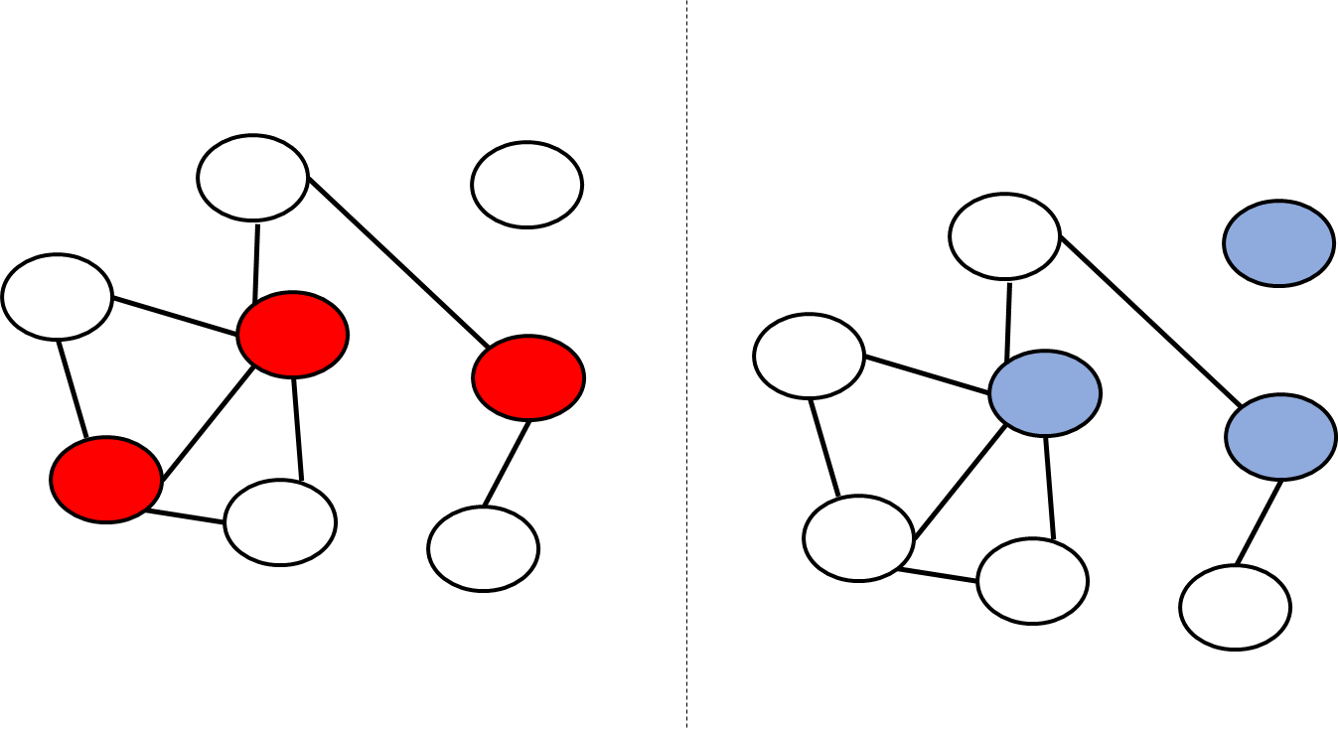
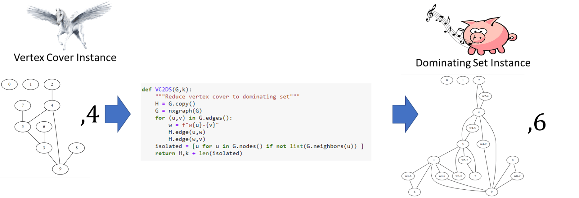
Since we know that \(\ensuremath{\mathit{ISET}} \leq_p \ensuremath{\mathit{VC}}\), using transitivity, it is enough to show that \(\ensuremath{\mathit{VC}} \leq_p \ensuremath{\mathit{DS}}\). As Figure 14.7 shows, a dominating set is not the same thing as a vertex cover. However, we can still relate the two problems. The idea is to map a graph \(G\) into a graph \(H\) such that a vertex cover in \(G\) would translate into a dominating set in \(H\) and vice versa. We do so by including in \(H\) all the vertices and edges of \(G\), but for every edge \(\{u ,v \}\) of \(G\) we also add to \(H\) a new vertex \(w_{u,v}\) and connect it to both \(u\) and \(v\). Let \(\ell\) be the number of isolated vertices in \(G\). The idea behind the proof is that we can transform a vertex cover \(S\) of \(k\) vertices in \(G\) into a dominating set of \(k+\ell\) vertices in \(H\) by adding to \(S\) all the isolated vertices, and moreover we can transform every \(k+\ell\)-sized dominating set in \(H\) into a vertex cover in \(G\). We now give the details.
Description of the algorithm. Given an instance \((G,k)\) for the vertex cover problem, we will map \(G\) into an instance \((H,k')\) for the dominating set problem as follows (see Figure 14.8 for Python implementation):
Algorithm 14.10 VC to DS reduction
Input: Graph \(G=(V,E)\) and number \(k\).
Output: Graph \(H=(V',E')\) and number \(k'\), such that \(G\) has a vertex cover of size \(k\) iff \(H\) has a dominating set of size \(k'\), that is, \(DS(H,k') = VC(G,k)\).
Initialize \(V' \leftarrow V, E' \leftarrow E\)
for {every edge \(\{u,v\} \in E\)}
Add vertex \(w_{u,v}\) to \(V'\)
Add edges \(\{ u, w_{u,v} \}\), \(\{ v, w_{u,v} \}\) to \(E'\).
endfor
Let \(\ell \leftarrow\) number of isolated vertices in \(G\)
return \(( H=(V',E') \;,\; k+\ell)\)
Algorithm 14.10 runs in polynomial time, since the loop takes \(O(m)\) steps where \(m\) is the number of edges, with each step can be implemented in constant or at most linear time (depending on the representation of the graph \(H\)). Counting the number of isolated vertices in an \(n\) vertex graph \(G\) can be done in time \(O(n^2)\) if \(G\) is represented in the adjacency matrix representation and \(O(n)\) time if it is represented in the adjacency list representation. Regardless the algorithm runs in polynomial time.
To complete the proof we need to prove that for every \(G,k\), if \(H,k'\) is the output of Algorithm 14.10 on input \((G,k)\), then \(\ensuremath{\mathit{DS}}(H,k') = \ensuremath{\mathit{VC}}(G,k)\). We split the proof into two parts. The completeness part is that if \(\ensuremath{\mathit{VC}}(G,k)=1\) then \(\ensuremath{\mathit{DS}}(H,k')=1\). The soundness part is that if \(\ensuremath{\mathit{DS}}(H,k')=1\) then \(\ensuremath{\mathit{VC}}(G,k)=1\).
Completeness. Suppose that \(\ensuremath{\mathit{VC}}(G,k)=1\). Then there is a vertex cover \(S \subseteq V\) of at most \(k\) vertices. Let \(I\) be the set of isolated vertices in \(G\) and \(\ell\) be their number. Then \(|S \cup I| \leq k +\ell\). We claim that \(S \cup I\) is a dominating set in \(H\). Indeed for every vertex \(v\) of \(H\) there are three cases:
Case 1: \(v\) is an isolated vertex of \(G\). In this case \(v\) is in \(S \cup I\).
Case 2: \(v\) is a non-isolated vertex of \(G\) and hence there is an edge \(\{ u,v \}\) of \(G\) for some \(u\). In this case since \(S\) is a vertex cover, one of \(u,v\) has to be in \(S\), and hence either \(v\) or a neighbor of \(v\) has to be in \(S \subseteq S \cup I\).
Case 3: \(v\) is of the form \(w_{u,u'}\) for some two neighbors \(u,u'\) in \(G\). But then since \(S\) is a vertex cover, one of \(u,u'\) has to be in \(S\) and hence \(S\) contains a neighbor of \(v\).
We conclude that \(S \cup I\) is a dominating set of size at most \(k'=k +\ell\) in \(H'\) and hence under the assumption that \(\ensuremath{\mathit{VC}}(G,k)=1\), \(\ensuremath{\mathit{DS}}(H',k')=1\).
Soundness. Suppose that \(\ensuremath{\mathit{DS}}(H,k')=1\). Then there is a dominating set \(D\) of size at most \(k' = k +\ell\) in \(H\). For every edge \(\{ u,v \}\) in the graph \(G\), if \(D\) contains the vertex \(w_{u,v}\) then we remove this vertex and add \(u\) in its place. The only two neighbors of \(w_{u,v}\) are \(u\) and \(v\), and since \(u\) is a neighbor of both \(w_{u,v}\) and of \(v\), replacing \(w_{u,v}\) with \(u\) maintains the property that it is a dominating set. Moreover, this change cannot increase the size of \(D\). Thus following this modification, we can assume that \(D\) is a dominating set of at most \(k+\ell\) vertices that does not contain any vertices of the form \(w_{u,v}\).
Let \(I\) be the set of isolated vertices in \(G\). These vertices are also isolated in \(H\) and hence must be included in \(D\) (an isolated vertex must be in any dominating set, since it has no neighbors). We let \(S = D \setminus I\). Then \(|S| \leq I\). We claim that \(S\) is a vertex cover in \(G\). Indeed, for every edge \(\{u,v\}\) of \(G\), either the vertex \(w_{u,v}\) or one of its neighbors must be in \(S\) by the dominating set property. But since we ensured \(S\) doesn’t contain any of the vertices of the form \(w_{u,v}\), it must be the case that either \(u\) or \(v\) is in \(S\). This shows that \(S\) is a vertex cover of \(G\) of size at most \(k\), hence proving that \(\ensuremath{\mathit{VC}}(G,k)=1\).
A corollary of Algorithm 14.10 and the other reduction we have seen so far is that if \(\ensuremath{\mathit{DS}} \in \mathbf{P}\) (i.e., dominating set has a polynomial-time algorithm) then \(3\ensuremath{\mathit{SAT}} \in \mathbf{P}\) (i.e., \(3\ensuremath{\mathit{SAT}}\) has a polynomial-time algorithm). By the contra-positive, if \(3\ensuremath{\mathit{SAT}}\) does not have a polynomial-time algorithm then neither does dominating set.
Anatomy of a reduction
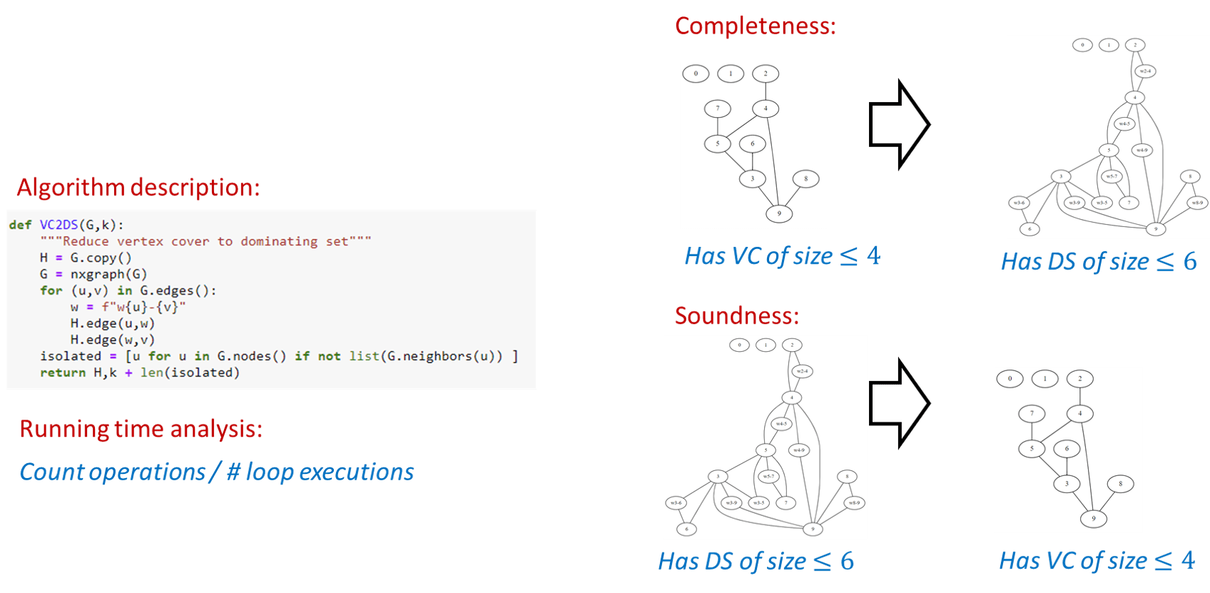
The reduction of Solved Exercise 14.5 gives a good illustration of the anatomy of a reduction. A reduction consists of four parts:
Algorithm description: This is the description of how the algorithm maps an input into the output. For example, in Solved Exercise 14.5 this is the description of how we map an instance \((G,k)\) of the vertex cover problem into an instance \((H,k')\) of the dominating set problem.
Algorithm analysis: It is not enough to describe how the algorithm works but we need to also explain why it works. In particular we need to provide an analysis explaining why the reduction is both efficient (i.e., runs in polynomial time) and correct (satisfies that \(G(R(x))=F(x)\) for every \(x\)). Specifically, the components of analysis of a reduction \(R\) include:
Efficiency: We need to show that \(R\) runs in polynomial time. In most reductions we encounter this part is straightforward, as the reductions we typically use involve a constant number of nested loops, each involving a constant number of operations. For example, the reduction of Solved Exercise 14.5 just enumerates over the edges and vertices of the input graph.
Completeness: In a reduction \(R\) demonstrating \(F \leq_p G\), the completeness condition is the condition that for every \(x\in \{0,1\}^*\), if \(F(x) = 1\) then \(G(R(x))=1\). Typically we construct the reduction to ensure that this holds, by giving a way to map a “certificate/solution” certifying that \(F(x)=1\) into a solution certifying that \(G(R(x))=1\). For example, in Solved Exercise 14.5 we constructed the graph \(H\) such that for every vertex cover \(S\) in \(G\), the set \(S \cup I\) (where \(I\) is the isolated vertices) would be a dominating set in \(H\).
Soundness: This is the condition that if \(F(x)=0\) then \(G(R(x))=0\) or (taking the contrapositive) if \(G(R(x))=1\) then \(F(x)=1\). This is sometimes straightforward but can often be harder to show than the completeness condition, and in more advanced reductions (such as the reduction \(3\ensuremath{\mathit{SAT}} \leq_p \ensuremath{\mathit{ISET}}\) of Theorem 14.8) demonstrating soundness is the main part of the analysis. For example, in Solved Exercise 14.5 to show soundness we needed to show that for every dominating set \(D\) in the graph \(H\), there exists a vertex cover \(S\) of size at most \(|D|-\ell\) in the graph \(G\) (where \(\ell\) is the number of isolated vertices). This was challenging since the dominating set \(D\) might not be necessarily the one we “had in mind”. In particular, in the proof above we needed to modify \(D\) to ensure that it does not contain vertices of the form \(w_{u,v}\), and it was important to show that this modification still maintains the property that \(D\) is a dominating set, and also does not make it bigger.
Whenever you need to provide a reduction, you should make sure that your description has all these components. While it is sometimes tempting to weave together the description of the reduction and its analysis, it is usually clearer if you separate the two, and also break down the analysis to its three components of efficiency, completeness, and soundness.
Reducing Independent Set to Maximum Cut
We now show that the independent set problem reduces to the maximum cut (or “max cut”) problem, modeled as the function \(\ensuremath{\mathit{MAXCUT}}\) that on input a pair \((G,k)\) outputs \(1\) iff \(G\) contains a cut of at least \(k\) edges. Since both are graph problems, a reduction from independent set to max cut maps one graph into the other, but as we will see the output graph does not have to have the same vertices or edges as the input graph.
\(\ensuremath{\mathit{ISET}} \leq_p \ensuremath{\mathit{MAXCUT}}\)
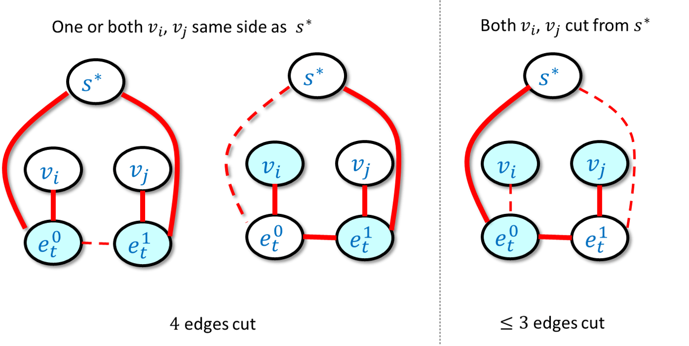
We will map a graph \(G\) into a graph \(H\) such that a large independent set in \(G\) becomes a partition cutting many edges in \(H\). We can think of a cut in \(H\) as coloring each vertex either “blue” or “red”. We will add a special “source” vertex \(s^*\), connect it to all other vertices, and assume without loss of generality that it is colored blue. Hence the more vertices we color red, the more edges from \(s^*\) we cut. Now, for every edge \(u,v\) in the original graph \(G\) we will add a special “gadget” which will be a small subgraph that involves \(u\),\(v\), the source \(s^*\), and two other additional vertices. We design the gadget in a way so that if the red vertices are not an independent set in \(G\) then the corresponding cut in \(H\) will be “penalized” in the sense that it would not cut as many edges. Once we set for ourselves this objective, it is not hard to find a gadget that achieves it\(-\) see the proof below. Once again the takeaway technique is to use (this time a slightly more clever) gadget.
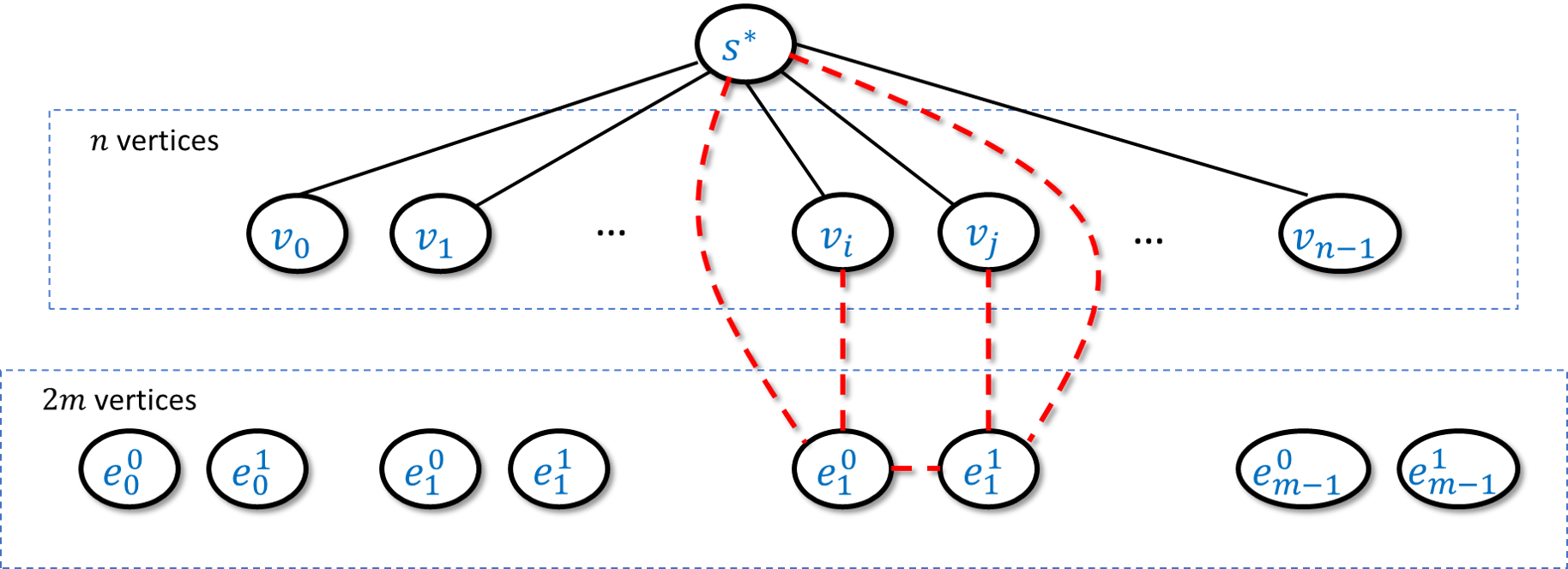
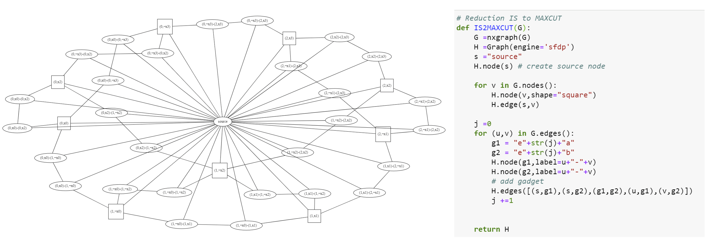
We will transform a graph \(G\) of \(n\) vertices and \(m\) edges into a graph \(H\) of \(n+1+2m\) vertices and \(n+5m\) edges in the following way (see also Figure 14.10). The graph \(H\) contains all vertices of \(G\) (though not the edges between them!) and in addition \(H\) also has:
* A special vertex \(s^*\) that is connected to all the vertices of \(G\)
* For every edge \(e=\{u,v\} \in E(G)\), two vertices \(e_0,e_1\) such that \(e_0\) is connected to \(u\) and \(e_1\) is connected to \(v\), and moreover we add the edges \(\{e_0,e_1 \},\{ e_0,s^* \},\{e_1,s^*\}\) to \(H\).
Theorem 14.11 will follow by showing that \(G\) contains an independent set of size at least \(k\) if and only if \(H\) has a cut cutting at least \(k+4m\) edges. We now prove both directions of this equivalence:
Part 1: Completeness. If \(I\) is an independent \(k\)-sized set in \(G\), then we can define \(S\) to be a cut in \(H\) of the following form: we let \(S\) contain all the vertices of \(I\) and for every edge \(e=\{u,v \} \in E(G)\), if \(u\in I\) and \(v\not\in I\) then we add \(e_1\) to \(S\); if \(u\not\in I\) and \(v\in I\) then we add \(e_0\) to \(S\); and if \(u\not\in I\) and \(v\not\in I\) then we add both \(e_0\) and \(e_1\) to \(S\). (We don’t need to worry about the case that both \(u\) and \(v\) are in \(I\) since it is an independent set.) We can verify that in all cases the number of edges from \(S\) to its complement in the gadget corresponding to \(e\) will be four (see Figure 14.11). Since \(s^*\) is not in \(S\), we also have \(k\) edges from \(s^*\) to \(I\), for a total of \(k+4m\) edges.
Part 2: Soundness. Suppose that \(S\) is a cut in \(H\) that cuts at least \(C=k+4m\) edges. We can assume that \(s^*\) is not in \(S\) (otherwise we can “flip” \(S\) to its complement \(\overline{S}\), since this does not change the size of the cut). Now let \(I\) be the set of vertices in \(S\) that correspond to the original vertices of \(G\). If \(I\) was an independent set of size \(k\) then we would be done. This might not always be the case but we will see that if \(I\) is not an independent set then it’s also larger than \(k\). Specifically, we define \(m_{in}=|E(I,I)|\) be the set of edges in \(G\) that are contained in \(I\) and let \(m_{out}=m-m_{in}\) (i.e., if \(I\) is an independent set then \(m_{in}=0\) and \(m_{out}=m\)). By the properties of our gadget we know that for every edge \(\{u,v\}\) of \(G\), we can cut at most three edges when both \(u\) and \(v\) are in \(S\), and at most four edges otherwise. Hence the number \(C\) of edges cut by \(S\) satisfies \(C \leq |I| + 3m_{in}+4m_{out} = |I|+ 3m_{in} + 4(m-m_{in})=|I|+4m-m_{in}\). Since \(C = k +4m\) we get that \(|I|-m_{in} \geq k\). Now we can transform \(I\) into an independent set \(I'\) by going over every one of the \(m_{in}\) edges that are inside \(I\) and removing one of the endpoints of the edge from it. The resulting set \(I'\) is an independent set in the graph \(G\) of size \(|I|-m_{in} \geq k\) and so this concludes the proof of the soundness condition.
Reducing 3SAT to Longest Path
Note: This section is still a little messy; feel free to skip it or just read it without going into the proof details. The proof appears in Section 7.5 in Sipser’s book.
One of the most basic algorithms in Computer Science is Dijkstra’s algorithm to find the shortest path between two vertices. We now show that in contrast, an efficient algorithm for the longest path problem would imply a polynomial-time algorithm for 3SAT.
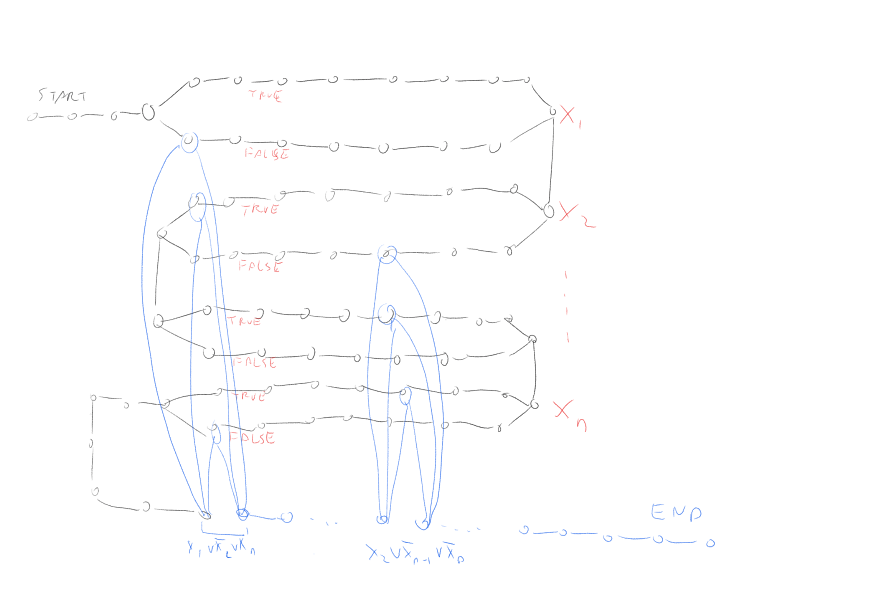
True) or the “lower path” (corresponding to assigning it the value False). Then to achieve maximum length the path would traverse through the blue part, where to go between two vertices corresponding to a clause such as \(x_{17} \vee \overline{x}_{32} \vee x_{57}\), the corresponding vertices would have to have been not traversed before.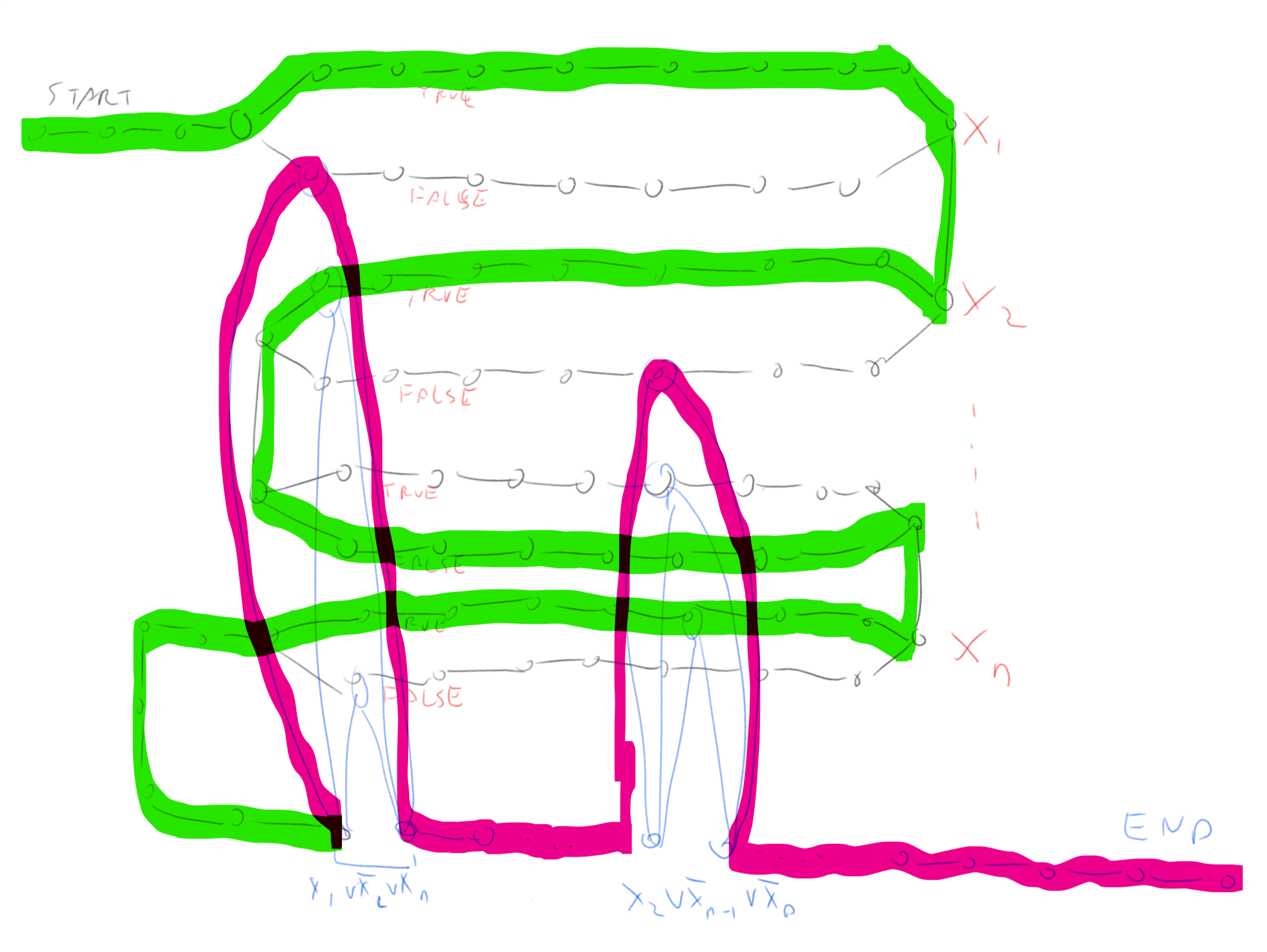
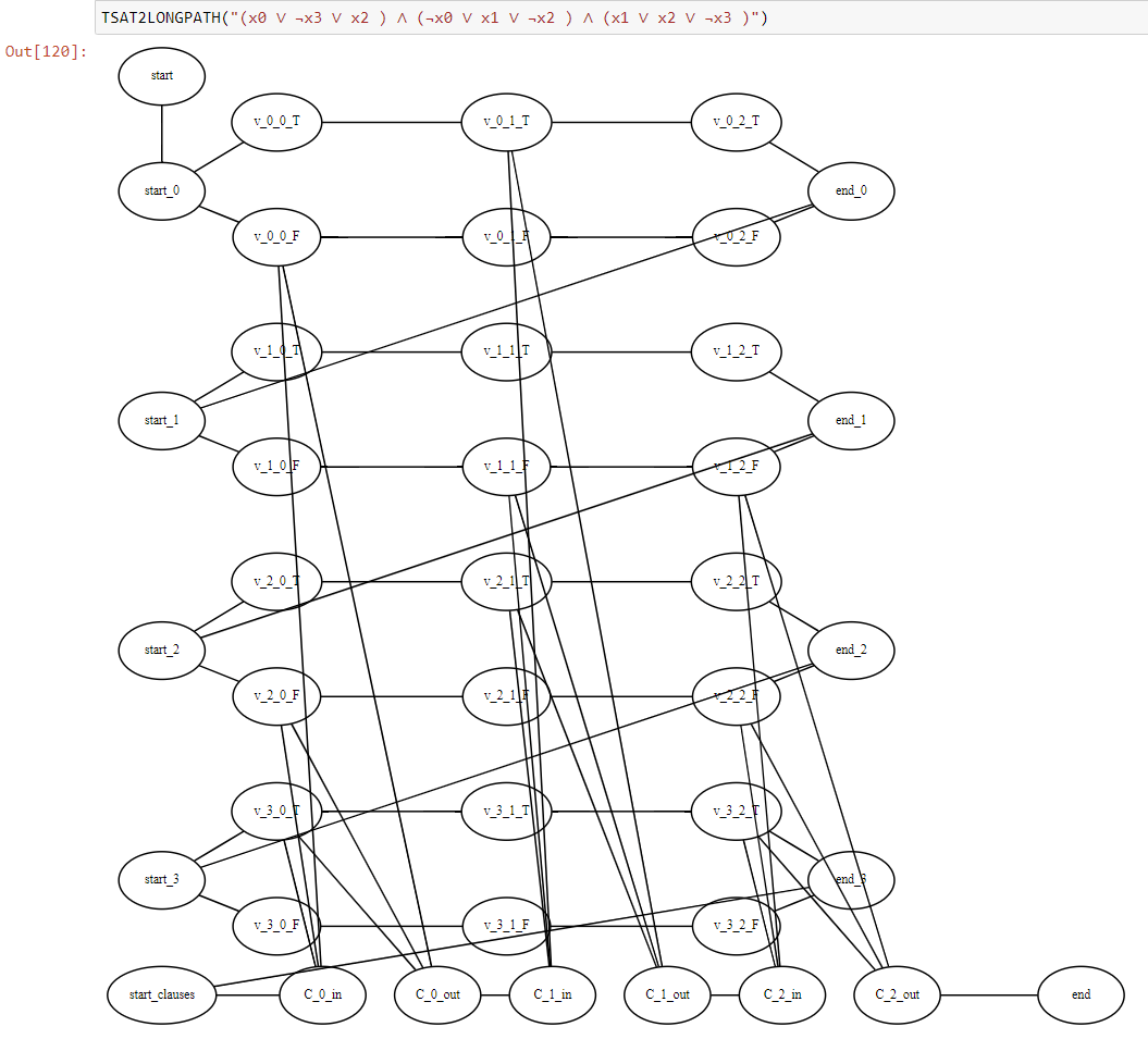
To prove Theorem 14.12 need to show how to transform a 3CNF formula \(\varphi\) into a graph \(G\) and two vertices \(s,t\) such that \(G\) has a path of length at least \(k\) if and only if \(\varphi\) is satisfiable. The idea of the reduction is sketched in Figure 14.13 and Figure 14.14. We will construct a graph that contains a potentially long “snaking path” that corresponds to all variables in the formula. We will add a “gadget” corresponding to each clause of \(\varphi\) in a way that we would only be able to use the gadgets if we have a satisfying assignment.
def TSAT2LONGPATH(φ):
    """Reduce 3SAT to LONGPATH"""
    def var(v): # return variable and True/False depending if positive or negated
        return int(v[2:]),False if v[0]=="¬" else int(v[1:]),True
    n = numvars(φ)
    clauses = getclauses(φ)
    m = len(clauses)
    G =Graph()
    G.edge("start","start_0")
    for i in range(n): # add 2 length-m paths per variable
        G.edge(f"start_{i}",f"v_{i}_{0}_T")
        G.edge(f"start_{i}",f"v_{i}_{0}_F")
        for j in range(m-1):
            G.edge(f"v_{i}_{j}_T",f"v_{i}_{j+1}_T")
            G.edge(f"v_{i}_{j}_F",f"v_{i}_{j+1}_F")
        G.edge(f"v_{i}_{m-1}_T",f"end_{i}")
        G.edge(f"v_{i}_{m-1}_F",f"end_{i}")
        if i<n-1:
            G.edge(f"end_{i}",f"start_{i+1}")
    G.edge(f"end_{n-1}","start_clauses")
    for j,C in enumerate(clauses): # add gadget for each clause
        for v in enumerate(C):
            i,sign = var(v[1])
            s = "F" if sign else "T"
            G.edge(f"C_{j}_in",f"v_{i}_{j}_{s}")
            G.edge(f"v_{i}_{j}_{s}",f"C_{j}_out")
        if j<m-1:
            G.edge(f"C_{j}_out",f"C_{j+1}_in")
    G.edge("start_clauses","C_0_in")
    G.edge(f"C_{m-1}_out","end")
    return G, 1+n*(m+1)+1+2*m+1
We build a graph \(G\) that “snakes” from \(s\) to \(t\) as follows. After \(s\) we add a sequence of \(n\) long loops. Each loop has an “upper path” and a “lower path”. A simple path cannot take both the upper path and the lower path, and so it will need to take exactly one of them to reach \(s\) from \(t\).
Our intention is that a path in the graph will correspond to an assignment \(x\in \{0,1\}^n\) in the sense that taking the upper path in the \(i^{th}\) loop corresponds to assigning \(x_i=1\) and taking the lower path corresponds to assigning \(x_i=0\). When we are done snaking through all the \(n\) loops corresponding to the variables to reach \(t\) we need to pass through \(m\) “obstacles”: for each clause \(j\) we will have a small gadget consisting of a pair of vertices \(s_j,t_j\) that have three paths between them. For example, if the \(j^{th}\) clause had the form \(x_{17} \vee \overline{x}_{55} \vee x_{72}\) then one path would go through a vertex in the lower loop corresponding to \(x_{17}\), one path would go through a vertex in the upper loop corresponding to \(x_{55}\) and the third would go through the lower loop corresponding to \(x_{72}\). We see that if we went in the first stage according to a satisfying assignment then we will be able to find a free vertex to travel from \(s_j\) to \(t_j\). We link \(t_1\) to \(s_2\), \(t_2\) to \(s_3\), etc and link \(t_m\) to \(t\). Thus a satisfying assignment would correspond to a path from \(s\) to \(t\) that goes through one path in each loop corresponding to the variables, and one path in each loop corresponding to the clauses. We can make the loop corresponding to the variables long enough so that we must take the entire path in each loop in order to have a fighting chance of getting a path as long as the one corresponds to a satisfying assignment. But if we do that, then the only way if we are able to reach \(t\) is if the paths we took corresponded to a satisfying assignment, since otherwise we will have one clause \(j\) where we cannot reach \(t_j\) from \(s_j\) without using a vertex we already used before.
Summary of relations
We have shown that there are a number of functions \(F\) for which we can prove a statement of the form “If \(F\in \mathbf{P}\) then \(3\ensuremath{\mathit{SAT}} \in \mathbf{P}\)”. Hence coming up with a polynomial-time algorithm for even one of these problems will entail a polynomial-time algorithm for \(3\ensuremath{\mathit{SAT}}\) (see for example Figure 14.16). In Chapter 15 we will show the inverse direction (“If \(3\ensuremath{\mathit{SAT}} \in \mathbf{P}\) then \(F\in \mathbf{P}\)”) for these functions, hence allowing us to conclude that they have equivalent complexity to \(3\ensuremath{\mathit{SAT}}\).

The computational complexity of many seemingly unrelated computational problems can be related to one another through the use of reductions.
If \(F \leq_p G\) then a polynomial-time algorithm for \(G\) can be transformed into a polynomial-time algorithm for \(F\).
Equivalently, if \(F \leq_p G\) and \(F\) does not have a polynomial-time algorithm then neither does \(G\).
We’ve developed many techniques to show that \(3\ensuremath{\mathit{SAT}} \leq_p F\) for interesting functions \(F\). Sometimes we can do so by using transitivity of reductions: if \(3\ensuremath{\mathit{SAT}} \leq_p G\) and \(G \leq_p F\) then \(3\ensuremath{\mathit{SAT}} \leq_p F\).
Exercises
Bibliographical notes
Several notions of reductions are defined in the literature. The notion defined in Definition 14.1 is often known as a mapping reduction, many to one reduction or a Karp reduction.
The maximal (as opposed to maximum) independent set is the task of finding a “local maximum” of an independent set: an independent set \(S\) such that one cannot add a vertex to it without losing the independence property (such a set is known as a vertex cover). Unlike finding a maximum independent set, finding a maximal independent set can be done efficiently by a greedy algorithm, but this local maximum can be much smaller than the global maximum.
Reduction of independent set to max cut taken from these notes. Image of Hamiltonian Path through Dodecahedron by Christoph Sommer.
We have mentioned that the line between reductions used for algorithm design and showing hardness is sometimes blurry. An excellent example for this is the area of SAT Solvers (see (Gomes, Kautz, Sabharwal, Selman, 2008) ). In this field people use algorithms for SAT (that take exponential time in the worst case but often are much faster on many instances in practice) together with reductions of the form \(F \leq_p \ensuremath{\mathit{SAT}}\) to derive algorithms for other functions \(F\) of interest.
- ↩
If you are familiar with matrix notation you may note that such equations can be written as \(Ax = \mathbf{b}\) where \(A\) is an \(m\times n\) matrix with entries in \(0/1\) and \(\mathbf{b} \in \N^m\).
Comments
Comments are posted on the GitHub repository using the utteranc.es app. A GitHub login is required to comment. If you don't want to authorize the app to post on your behalf, you can also comment directly on the GitHub issue for this page.
Compiled on 12/06/2023 00:07:22
Copyright 2023, Boaz Barak.

This work is
licensed under a Creative Commons
Attribution-NonCommercial-NoDerivatives 4.0 International License.
Produced using pandoc and panflute with templates derived from gitbook and bookdown.