See any bugs/typos/confusing explanations? Open a GitHub issue. You can also comment below
★ See also the PDF version of this chapter (better formatting/references) ★
Functions with Infinite domains, Automata, and Regular expressions
- Define functions on unbounded length inputs, that cannot be described by a finite size table of inputs and outputs.
- Equivalence with the task of deciding membership in a language.
- Deterministic finite automatons (optional): A simple example for a model for unbounded computation.
- Equivalence with regular expressions.
“An algorithm is a finite answer to an infinite number of questions.”, Attributed to Stephen Kleene.
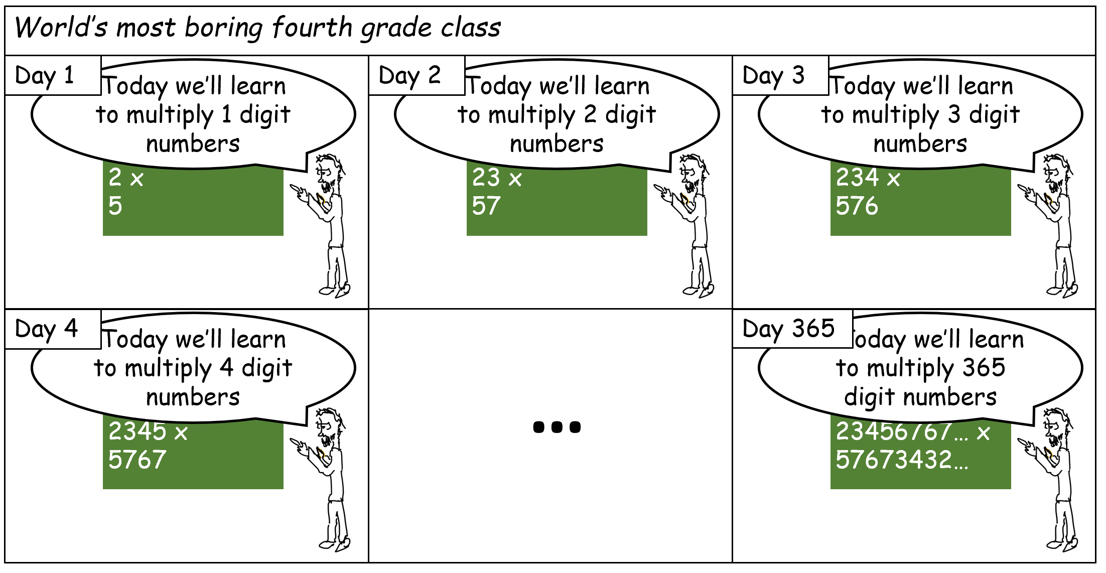
The model of Boolean circuits (or equivalently, the NAND-CIRC programming language) has one very significant drawback: a Boolean circuit can only compute a finite function \(f\). In particular, since every gate has two inputs, a size \(s\) circuit can compute on an input of length at most \(2s\). Thus this model does not capture our intuitive notion of an algorithm as a single recipe to compute a potentially infinite function. For example, the standard elementary school multiplication algorithm is a single algorithm that multiplies numbers of all lengths. However, we cannot express this algorithm as a single circuit, but rather need a different circuit (or equivalently, a NAND-CIRC program) for every input length (see Figure 6.1).
In this chapter, we extend our definition of computational tasks to consider functions with the unbounded domain of \(\{0,1\}^*\). We focus on the question of defining what tasks to compute, mostly leaving the question of how to compute them to later chapters, where we will see Turing machines and other computational models for computing on unbounded inputs. However, we will see one example of a simple restricted model of computation - deterministic finite automata (DFAs).
In this chapter, we discuss functions that take as input strings of arbitrary length. We will often focus on the special case of Boolean functions, where the output is a single bit. These are still infinite functions since their inputs have unbounded length and hence such a function cannot be computed by any single Boolean circuit.
In the second half of this chapter, we discuss finite automata, a computational model that can compute unbounded length functions. Finite automata are not as powerful as Python or other general-purpose programming languages but can serve as an introduction to these more general models. We also show a beautiful result - the functions computable by finite automata are precisely the ones that correspond to regular expressions. However, the reader can also feel free to skip automata and go straight to our discussion of Turing machines in Chapter 7.
Functions with inputs of unbounded length
Up until now, we considered the computational task of mapping some string of length \(n\) into a string of length \(m\). However, in general, computational tasks can involve inputs of unbounded length. For example, the following Python function computes the function \(\ensuremath{\mathit{XOR}}:\{0,1\}^* \rightarrow \{0,1\}\), where \(\ensuremath{\mathit{XOR}}(x)\) equals \(1\) iff the number of \(1\)’s in \(x\) is odd. (In other words, \(\ensuremath{\mathit{XOR}}(x) = \sum_{i=0}^{|x|-1} x_i \mod 2\) for every \(x\in \{0,1\}^*\).) As simple as it is, the \(\ensuremath{\mathit{XOR}}\) function cannot be computed by a Boolean circuit. Rather, for every \(n\), we can compute \(\ensuremath{\mathit{XOR}}_n\) (the restriction of \(\ensuremath{\mathit{XOR}}\) to \(\{0,1\}^n\)) using a different circuit (e.g., see Figure 6.2).
def XOR(X):
    '''Takes list X of 0's and 1's
       Outputs 1 if the number of 1's is odd and outputs 0 otherwise'''
    result = 0
    for i in range(len(X)):
        result = (result + X[i]) % 2
    return result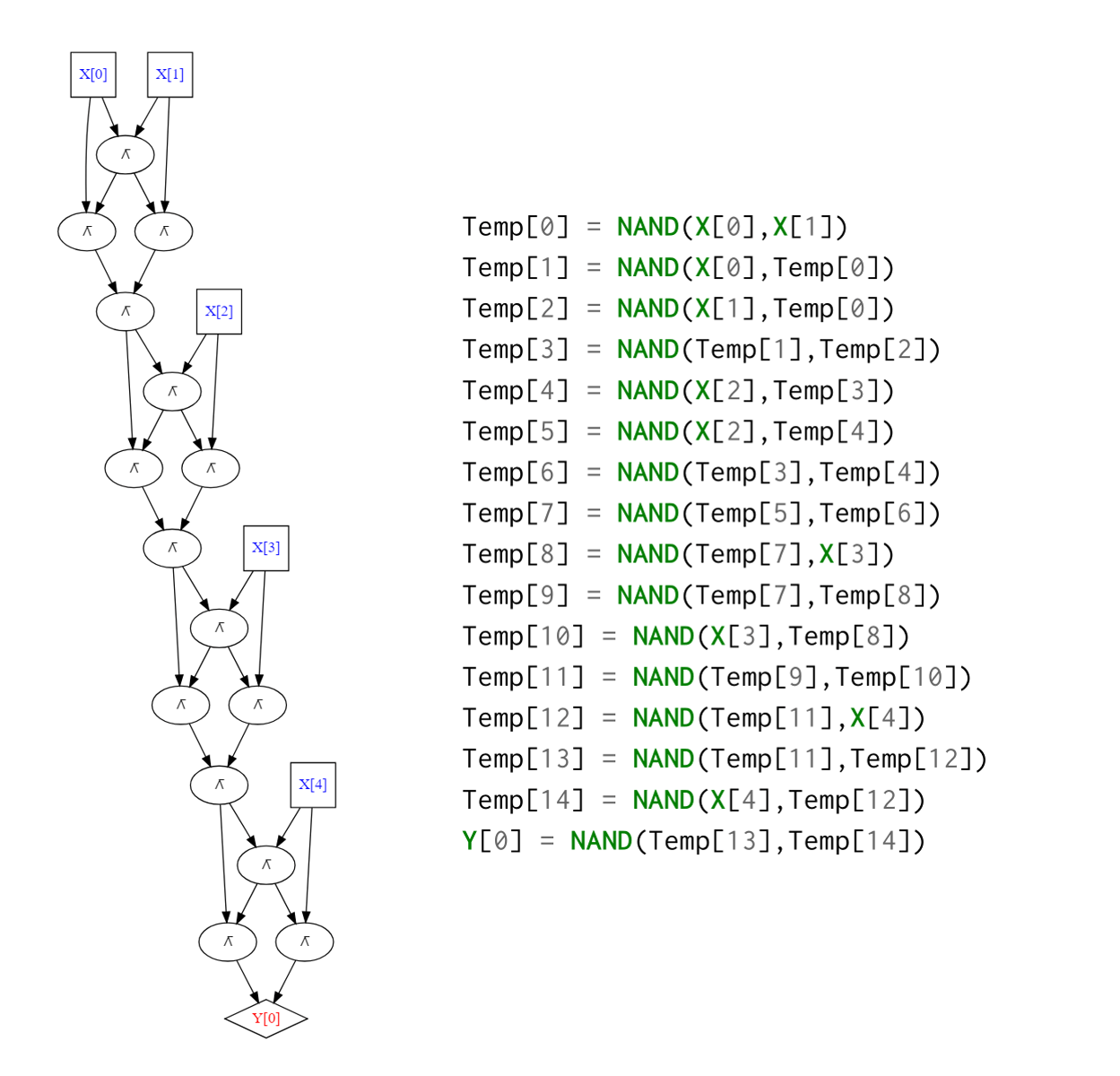
Previously in this book, we studied the computation of finite functions \(f:\{0,1\}^n \rightarrow \{0,1\}^m\). Such a function \(f\) can always be described by listing all the \(2^n\) values it takes on inputs \(x\in \{0,1\}^n\). In this chapter, we consider functions such as \(\ensuremath{\mathit{XOR}}\) that take inputs of unbounded size. While we can describe \(\ensuremath{\mathit{XOR}}\) using a finite number of symbols (in fact, we just did so above), it takes infinitely many possible inputs, and so we cannot just write down all of its values. The same is true for many other functions capturing important computational tasks, including addition, multiplication, sorting, finding paths in graphs, fitting curves to points, and so on. To contrast with the finite case, we will sometimes call a function \(F:\{0,1\}^* \rightarrow \{0,1\}\) (or \(F:\{0,1\}^* \rightarrow \{0,1\}^*\)) infinite. However, this does not mean that \(F\) takes as input strings of infinite length! It just means that \(F\) can take as input a string that can be arbitrarily long, and so we cannot simply write down a table of all the outputs of \(F\) on different inputs.
A function \(F:\{0,1\}^* \rightarrow \{0,1\}^*\) specifies the computational task mapping an input \(x\in \{0,1\}^*\) into the output \(F(x)\).
As we have seen before, restricting attention to functions that use binary strings as inputs and outputs does not detract from our generality, since other objects, including numbers, lists, matrices, images, videos, and more, can be encoded as binary strings.
As before, it is essential to differentiate between specification and implementation. For example, consider the following function:
This is a mathematically well-defined function. For every \(x\), \(\ensuremath{\mathit{TWINP}}(x)\) has a unique value which is either \(0\) or \(1\). However, at the moment, no one knows of a Python program that computes this function. The Twin prime conjecture posits that for every \(n\) there exists \(p>n\) such that both \(p\) and \(p+2\) are primes. If this conjecture is true, then \(T\) is easy to compute indeed - the program def T(x): return 1 will do the trick. However, mathematicians have tried unsuccessfully to prove this conjecture since 1849. That said, whether or not we know how to implement the function \(\ensuremath{\mathit{TWINP}}\), the definition above provides its specification.
Varying inputs and outputs
Many of the functions that interest us take more than one input. For example, the function
takes the binary representation of a pair of integers \(x,y \in \N\), and outputs the binary representation of their product \(x \cdot y\). However, since we can represent a pair of strings as a single string, we will consider functions such as MULT as mapping \(\{0,1\}^*\) to \(\{0,1\}^*\). We will typically not be concerned with low-level details such as the precise way to represent a pair of integers as a string, since virtually all choices will be equivalent for our purposes.
Another example of a function we want to compute is
\(\ensuremath{\mathit{PALINDROME}}\) has a single bit as output. Functions with a single bit of output are known as Boolean functions. Boolean functions are central to the theory of computation, and we will discuss them often in this book. Note that even though Boolean functions have a single bit of output, their input can be of arbitrary length. Thus they are still infinite functions that cannot be described via a finite table of values.
“Booleanizing” functions. Sometimes it might be convenient to obtain a Boolean variant for a non-Boolean function. For example, the following is a Boolean variant of \(\ensuremath{\mathit{MULT}}\).
If we can compute \(\ensuremath{\mathit{BMULT}}\) via any programming language such as Python, C, Java, etc., we can compute \(\ensuremath{\mathit{MULT}}\) as well, and vice versa.
Show that for every function \(F:\{0,1\}^* \rightarrow \{0,1\}^*\), there exists a Boolean function \(\ensuremath{\mathit{BF}}:\{0,1\}^* \rightarrow \{0,1\}\) such that a Python program to compute \(\ensuremath{\mathit{BF}}\) can be transformed into a program to compute \(F\) and vice versa.
For every \(F:\{0,1\}^* \rightarrow \{0,1\}^*\), we can define
to be the function that on input \(x \in \{0,1\}^*, i \in \N, b\in \{0,1\}\) outputs the \(i^{th}\) bit of \(F(x)\) if \(b=0\) and \(i<|F(x)|\). If \(b=1\), then \(\ensuremath{\mathit{BF}}(x,i,b)\) outputs \(1\) iff \(i<|F(x)|\) and hence this allows to compute the length of \(F(x)\).
Computing \(\ensuremath{\mathit{BF}}\) from \(F\) is straightforward. For the other direction, given a Python function BF that computes \(\ensuremath{\mathit{BF}}\), we can compute \(F\) as follows:
Formal Languages
For every Boolean function \(F:\{0,1\}^* \rightarrow \{0,1\}\), we can define the set \(L_F = \{ x | F(x) = 1 \}\) of strings on which \(F\) outputs \(1\). Such sets are known as languages. This name is rooted in formal language theory as pursued by linguists such as Noam Chomsky. A formal language is a subset \(L \subseteq \{0,1\}^*\) (or more generally \(L \subseteq \Sigma^*\) for some finite alphabet \(\Sigma\)). The membership or decision problem for a language \(L\), is the task of determining, given \(x\in \{0,1\}^*\), whether or not \(x\in L\). If we can compute the function \(F\), then we can decide membership in the language \(L_F\) and vice versa. Hence, many texts such as (Sipser, 1997) refer to the task of computing a Boolean function as “deciding a language”. In this book, we mostly describe computational tasks using the function notation, which is easier to generalize to computation with more than one bit of output. However, since the language terminology is so popular in the literature, we will sometimes mention it.
Restrictions of functions
If \(F:\{0,1\}^* \rightarrow \{0,1\}\) is a Boolean function and \(n\in \N\) then the restriction of \(F\) to inputs of length \(n\), denoted as \(F_n\), is the finite function \(f:\{0,1\}^n \rightarrow \{0,1\}\) such that \(f(x) = F(x)\) for every \(x\in \{0,1\}^n\). That is, \(F_n\) is the finite function that is only defined on inputs in \(\{0,1\}^n\), but agrees with \(F\) on those inputs. Since \(F_n\) is a finite function, it can be computed by a Boolean circuit, implying the following theorem:
Let \(F:\{0,1\}^* \rightarrow \{0,1\}\). Then there is a collection \(\{ C_n \}_{n\in \{1,2,\ldots\}}\) of circuits such that for every \(n>0\), \(C_n\) computes the restriction \(F_n\) of \(F\) to inputs of length \(n\).
This is an immediate corollary of the universality of Boolean circuits. Indeed, since \(F_n\) maps \(\{0,1\}^n\) to \(\{0,1\}\), Theorem 4.15 implies that there exists a Boolean circuit \(C_n\) to compute it. In fact, the size of this circuit is at most \(c \cdot 2^n / n\) gates for some constant \(c \leq 10\).
In particular, Theorem 6.1 implies that there exists such a circuit collection \(\{ C_n \}\) even for the \(\ensuremath{\mathit{TWINP}}\) function we described before, even though we do not know of any program to compute it. Indeed, this is not that surprising: for every particular \(n\in \N\), \(\ensuremath{\mathit{TWINP}}_n\) is either the constant zero function or the constant one function, both of which can be computed by very simple Boolean circuits. Hence a collection of circuits \(\{ C_n \}\) that computes \(\ensuremath{\mathit{TWINP}}\) certainly exists. The difficulty in computing \(\ensuremath{\mathit{TWINP}}\) using Python or any other programming language arises from the fact that we do not know for each particular \(n\) what is the circuit \(C_n\) in this collection.
Deterministic finite automata (optional)
All our computational models so far - Boolean circuits and straight-line programs - were only applicable for finite functions.
In Chapter 7, we will present Turing machines, which are the central models of computation for unbounded input length functions. However, in this section we present the more basic model of deterministic finite automata (DFA). Automata can serve as a good stepping-stone for Turing machines, though they will not be used much in later parts of this book, and so the reader can feel free to skip ahead to Chapter 7. DFAs turn out to be equivalent in power to regular expressions: a powerful mechanism to specify patterns, which is widely used in practice. Our treatment of automata is relatively brief. There are plenty of resources that help you get more comfortable with DFAs. In particular, Chapter 1 of Sipser’s book (Sipser, 1997) contains an excellent exposition of this material. There are also many websites with online simulators for automata, as well as translators from regular expressions to automata and vice versa (see for example here and here).
At a high level, an algorithm is a recipe for computing an output from an input via a combination of the following steps:
- Read a bit from the input
- Update the state (working memory)
- Stop and produce an output
For example, recall the Python program that computes the \(\ensuremath{\mathit{XOR}}\) function:
def XOR(X):
'''Takes list X of 0's and 1's
Outputs 1 if the number of 1's is odd and outputs 0 otherwise'''
result = 0
for i in range(len(X)):
result = (result + X[i]) % 2
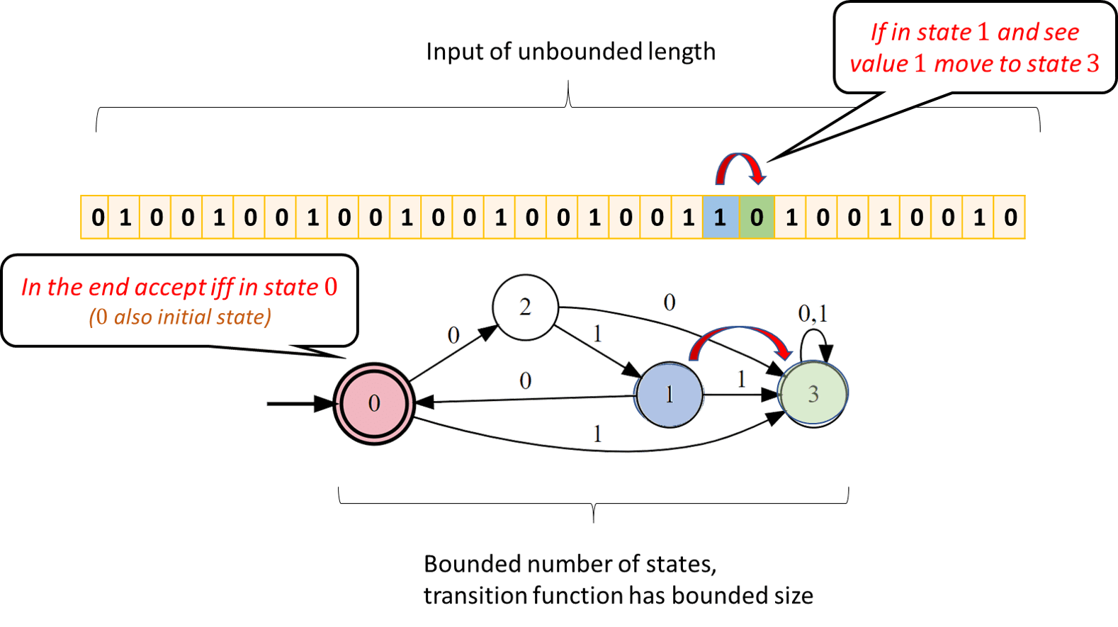
return resultIn each step, this program reads a single bit X[i] and updates its state result based on that bit (flipping result if X[i] is \(1\) and keeping it the same otherwise). When it is done transversing the input, the program outputs result. In computer science, such a program is called a single-pass constant-memory algorithm since it makes a single pass over the input and its working memory is finite. (Indeed, in this case, result can either be \(0\) or \(1\).) Such an algorithm is also known as a Deterministic Finite Automaton or DFA (another name for DFAs is a finite state machine). We can think of such an algorithm as a “machine” that can be in one of \(C\) states, for some constant \(C\). The machine starts in some initial state and then reads its input \(x\in \{0,1\}^*\) one bit at a time. Whenever the machine reads a bit \(\sigma \in \{0,1\}\), it transitions into a new state based on \(\sigma\) and its prior state. The output of the machine is based on the final state. Every single-pass constant-memory algorithm corresponds to such a machine. If an algorithm uses \(c\) bits of memory, then the contents of its memory can be represented as a string of length \(c\). Therefore such an algorithm can be in one of at most \(2^c\) states at any point in the execution.
We can specify a DFA of \(C\) states by a list of \(C \cdot 2\) rules. Each rule will be of the form “If the DFA is in state \(v\) and the bit read from the input is \(\sigma\) then the new state is \(v'\)”. At the end of the computation, we will also have a rule of the form “If the final state is one of the following … then output \(1\), otherwise output \(0\)”. For example, the Python program above can be represented by a two-state automaton for computing \(\ensuremath{\mathit{XOR}}\) of the following form:
- Initialize in the state \(0\).
- For every state \(s \in \{0,1\}\) and input bit \(\sigma\) read, if \(\sigma =1\) then change to state \(1-s\), otherwise stay in state \(s\).
- At the end output \(1\) iff \(s=1\).
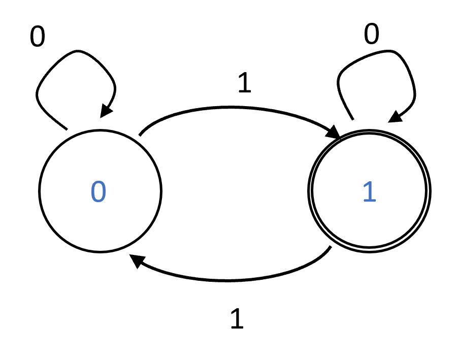
We can also describe a \(C\)-state DFA as a labeled graph of \(C\) vertices. For every state \(s\) and bit \(\sigma\), we add a directed edge labeled with \(\sigma\) between \(s\) and the state \(s'\) such that if the DFA is at state \(s\) and reads \(\sigma\) then it transitions to \(s'\). (If the state stays the same then this edge will be a self-loop; similarly, if \(s\) transitions to \(s'\) in both the case \(\sigma=0\) and \(\sigma=1\) then the graph will contain two parallel edges.) We also label the set \(\mathcal{S}\) of states on which the automaton will output \(1\) at the end of the computation. This set is known as the set of accepting states. See Figure 6.3 for the graphical representation of the XOR automaton.
Formally, a DFA is specified by (1) the table of the \(C \cdot 2\) rules, which can be represented as a transition function \(T\) that maps a state \(s \in [C]\) and bit \(\sigma \in \{0,1\}\) to the state \(s' \in [C]\) which the DFA will transition to from state \(s\) on input \(\sigma\) and (2) the set \(\mathcal{S}\) of accepting states. This leads to the following definition.
A deterministic finite automaton (DFA) with \(C\) states over \(\{0,1\}\) is a pair \((T,\mathcal{S})\) with \(T:[C]\times \{0,1\} \rightarrow [C]\) and \(\mathcal{S} \subseteq [C]\). The finite function \(T\) is known as the transition function of the DFA. The set \(\mathcal{S}\) is known as the set of accepting states.
Let \(F:\{0,1\}^* \rightarrow \{0,1\}\) be a Boolean function with the infinite domain \(\{0,1\}^*\). We say that \((T,\mathcal{S})\) computes a function \(F:\{0,1\}^* \rightarrow \{0,1\}\) if for every \(n\in\N\) and \(x\in \{0,1\}^n\), if we define \(s_0=0\) and \(s_{i+1} = T(s_i,x_i)\) for every \(i\in [n]\), then
Make sure not to confuse the transition function of an automaton (\(T\) in Definition 6.2), which is a finite function specifying the table of “rules” which it follows, with the function the automaton computes (\(F\) in Definition 6.2) which is an infinite function.
Deterministic finite automata can be defined in several equivalent ways. In particular Sipser (Sipser, 1997) defines a DFA as a five-tuple \((Q,\Sigma,\delta,q_0,F)\) where \(Q\) is the set of states, \(\Sigma\) is the alphabet, \(\delta\) is the transition function, \(q_0\) is the initial state, and \(F\) is the set of accepting states. In this book the set of states is always of the form \(Q=\{0,\ldots,C-1 \}\) and the initial state is always \(q_0 = 0\), but this makes no difference to the computational power of these models. Also, we restrict our attention to the case that the alphabet \(\Sigma\) is equal to \(\{0,1\}\).
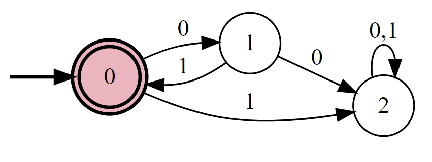
Prove that there is a DFA that computes the following function \(F\):
When asked to construct a deterministic finite automaton, it is often useful to start by constructing a single-pass constant-memory algorithm using a more general formalism (for example, using pseudocode or a Python program). Once we have such an algorithm, we can mechanically translate it into a DFA. Here is a simple Python program for computing \(F\):
def F(X):
'''Return 1 iff X is a concatenation of zero/more copies of [0,1,0]'''
if len(X) % 3 != 0:
return False
ultimate = 0
penultimate = 1
antepenultimate = 0
for idx, b in enumerate(X):
antepenultimate = penultimate
penultimate = ultimate
ultimate = b
if idx % 3 == 2 and ((antepenultimate, penultimate, ultimate) != (0,1,0)):
return False
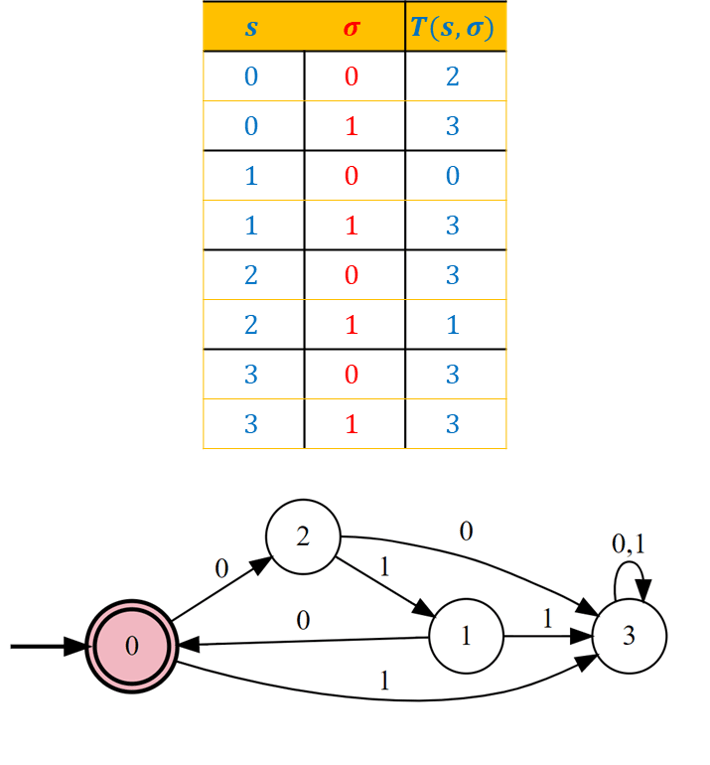
return TrueSince we keep three Boolean variables, the working memory can be in one of \(2^3 = 8\) configurations, and so the program above can be directly translated into an \(8\) state DFA. While this is not needed to solve the question, by examining the resulting DFA, we can see that we can merge some states and obtain a \(4\) state automaton, described in Figure 6.4. See also Figure 6.5, which depicts the execution of this DFA on a particular input.
Anatomy of an automaton (finite vs. unbounded)
Now that we are considering computational tasks with unbounded input sizes, it is crucial to distinguish between the components of our algorithm that have fixed length and the components that grow with the input size. For the case of DFAs these are the following:
Constant size components: Given a DFA \(A\), the following quantities are fixed independent of the input size:
The number of states \(C\) in \(A\).
The transition function \(T\) (which has \(2C\) inputs, and so can be specified by a table of \(2C\) rows, each entry in which is a number in \([C]\)).
The set \(\mathcal{S} \subseteq [C]\) of accepting states. This set can be described by a string in \(\{0,1\}^C\) specifiying which states are in \(\mathcal{S}\) and which are not.
Together the above means that we can fully describe an automaton using finitely many symbols. This is a property we require out of any notion of “algorithm”: we should be able to write down a complete specification of how it produces an output from an input.
Components of unbounded size: The following quantities relating to a DFA are not bounded by any constant. We stress that these are still finite for any given input.
The length of the input \(x\in \{0,1\}^*\) that the DFA is provided. The input length is always finite, but not a priori bounded.
The number of steps that the DFA takes can grow with the length of the input. Indeed, a DFA makes a single pass on the input and so it takes precisely \(|x|\) steps on an input \(x\in \{0,1\}^*\).
DFA-computable functions
We say that a function \(F:\{0,1\}^* \rightarrow \{0,1\}\) is DFA computable if there exists some \(\ensuremath{\mathit{DFA}}\) that computes \(F\). In Chapter 4 we saw that every finite function is computable by some Boolean circuit. Thus, at this point, you might expect that every infinite function is computable by some DFA. However, this is very much not the case. We will soon see some simple examples of infinite functions that are not computable by DFAs, but for starters, let us prove that such functions exist.
Let \(\ensuremath{\mathit{DFACOMP}}\) be the set of all Boolean functions \(F:\{0,1\}^* \rightarrow \{0,1\}\) such that there exists a DFA computing \(F\). Then \(\ensuremath{\mathit{DFACOMP}}\) is countable.
Every DFA can be described by a finite length string, which yields an onto map from \(\{0,1\}^*\) to \(\ensuremath{\mathit{DFACOMP}}\): namely, the function that maps a string describing an automaton \(A\) to the function that it computes.
Every DFA can be described by a finite string, representing the transition function \(T\) and the set of accepting states, and every DFA \(A\) computes some function \(F:\{0,1\}^* \rightarrow \{0,1\}\). Thus we can define the following function \(StDC:\{0,1\}^* \rightarrow \ensuremath{\mathit{DFACOMP}}\):
Since the set of all Boolean functions is uncountable, we get the following corollary:
There exists a Boolean function \(F:\{0,1\}^* \rightarrow \{0,1\}\) that is not computable by any DFA.
If every Boolean function \(F\) is computable by some DFA, then \(\ensuremath{\mathit{DFACOMP}}\) equals the set \(\ensuremath{\mathit{ALL}}\) of all Boolean functions, but by Theorem 2.12, the latter set is uncountable, contradicting Theorem 6.4.
Regular expressions
Searching for a piece of text is a common task in computing. At its heart, the search problem is quite simple. We have a collection \(X = \{ x_0, \ldots, x_k \}\) of strings (e.g., files on a hard-drive, or student records in a database), and the user wants to find out the subset of all the \(x \in X\) that are matched by some pattern (e.g., all files whose names end with the string .txt). In full generality, we can allow the user to specify the pattern by specifying a (computable) function \(F:\{0,1\}^* \rightarrow \{0,1\}\), where \(F(x)=1\) corresponds to the pattern matching \(x\). That is, the user provides a program \(P\) in a programming language such as Python, and the system returns all \(x \in X\) such that \(P(x)=1\). For example, one could search for all text files that contain the string important document or perhaps (letting \(P\) correspond to a neural-network based classifier) all images that contain a cat. However, we don’t want our system to get into an infinite loop just trying to evaluate the program \(P\)! For this reason, typical systems for searching files or databases do not allow users to specify the patterns using full-fledged programming languages. Rather, such systems use restricted computational models that on the one hand are rich enough to capture many of the queries needed in practice (e.g., all filenames ending with .txt, or all phone numbers of the form (617) xxx-xxxx), but on the other hand are restricted enough so that queries can be evaluated very efficiently on huge files and in particular cannot result in an infinite loop.
One of the most popular such computational models is regular expressions. If you ever used an advanced text editor, a command-line shell, or have done any kind of manipulation of text files, then you have probably come across regular expressions.
A regular expression over some alphabet \(\Sigma\) is obtained by combining elements of \(\Sigma\) with the operation of concatenation, as well as \(|\) (corresponding to or) and \(*\) (corresponding to repetition zero or more times). (Common implementations of regular expressions in programming languages and shells typically include some extra operations on top of \(|\) and \(*\), but these operations can be implemented as “syntactic sugar” using the operators \(|\) and \(*\).) For example, the following regular expression over the alphabet \(\{0,1\}\) corresponds to the set of all strings \(x\in \{0,1\}^*\) where every digit is repeated at least twice:
The following regular expression over the alphabet \(\{ a,\ldots,z,0,\ldots,9 \}\) corresponds to the set of all strings that consist of a sequence of one or more of the letters \(a\)-\(d\) followed by a sequence of one or more digits (without a leading zero):
Formally, regular expressions are defined by the following recursive definition:
A regular expression \(e\) over an alphabet \(\Sigma\) is a string over \(\Sigma \cup \{ (,),|,*,\emptyset, \ensuremath{\text{\texttt{""}}} \}\) that has one of the following forms:
\(e = \sigma\) where \(\sigma \in \Sigma\)
\(e = (e' | e'')\) where \(e', e''\) are regular expressions.
\(e = (e')(e'')\) where \(e',e''\) are regular expressions. (We often drop the parentheses when there is no danger of confusion and so write this as \(e' \; e''\).)
\(e = (e')^*\) where \(e'\) is a regular expression.
Finally we also allow the following “edge cases”: \(e = \emptyset\) and \(e = \ensuremath{\text{\texttt{""}}}\). These are the regular expressions corresponding to accepting no strings, and accepting only the empty string respectively.
We will drop parentheses when they can be inferred from the context. We also use the convention that OR and concatenation are left-associative, and we give highest precedence to \(*\), then concatenation, and then OR. Thus for example we write \(00^*|11\) instead of \(((0)(0^*))|((1)(1))\).
Every regular expression \(e\) corresponds to a function \(\Phi_{e}:\Sigma^* \rightarrow \{0,1\}\) where \(\Phi_{e}(x)=1\) if \(x\) matches the regular expression. For example, if \(e = (00|11)^*\) then \(\Phi_e(110011)=1\) but \(\Phi_e(101)=0\) (can you see why?).
The formal definition of \(\Phi_{e}\) is one of those definitions that is more cumbersome to write than to grasp. Thus it might be easier for you first to work out the definition on your own, and then check that it matches what is written below.
Let \(e\) be a regular expression over the alphabet \(\Sigma\). The function \(\Phi_{e}:\Sigma^* \rightarrow \{0,1\}\) is defined as follows:
If \(e = \sigma\) then \(\Phi_{e}(x)=1\) iff \(x=\sigma\).
If \(e = (e' | e'')\) then \(\Phi_{e}(x) = \Phi_{e'}(x) \vee \Phi_{e''}(x)\) where \(\vee\) is the OR operator.
If \(e = (e')(e'')\) then \(\Phi_{e}(x) = 1\) iff there is some \(x',x'' \in \Sigma^*\) such that \(x\) is the concatenation of \(x'\) and \(x''\) and \(\Phi_{e'}(x')=\Phi_{e''}(x'')=1\).
If \(e= (e')*\) then \(\Phi_{e}(x)=1\) iff there is some \(k\in \N\) and some \(x_0,\ldots,x_{k-1} \in \Sigma^*\) such that \(x\) is the concatenation \(x_0 \cdots x_{k-1}\) and \(\Phi_{e'}(x_i)=1\) for every \(i\in [k]\).
Finally, for the edge cases \(\Phi_{\emptyset}\) is the constant zero function, and \(\Phi_{\ensuremath{\text{\texttt{""}}}}\) is the function that only outputs \(1\) on the empty string \(\ensuremath{\text{\texttt{""}}}\).
We say that a regular expression \(e\) over \(\Sigma\) matches a string \(x \in \Sigma^*\) if \(\Phi_{e}(x)=1\).
The definitions above are not inherently difficult but are a bit cumbersome. So you should pause here and go over it again until you understand why it corresponds to our intuitive notion of regular expressions. This is important not just for understanding regular expressions themselves (which are used time and again in a great many applications) but also for getting better at understanding recursive definitions in general.
A Boolean function is called “regular” if it outputs \(1\) on precisely the set of strings that are matched by some regular expression. That is,
Let \(\Sigma\) be a finite set and \(F:\Sigma^* \rightarrow \{0,1\}\) be a Boolean function. We say that \(F\) is regular if \(F=\Phi_{e}\) for some regular expression \(e\).
Similarly, for every formal language \(L \subseteq \Sigma^*\), we say that \(L\) is regular if and only if there is a regular expression \(e\) such that \(x\in L\) iff \(e\) matches \(x\).
Let \(\Sigma=\{ a,b,c,d,0,1,2,3,4,5,6,7,8,9 \}\) and \(F:\Sigma^* \rightarrow \{0,1\}\) be the function such that \(F(x)\) outputs \(1\) iff \(x\) consists of one or more of the letters \(a\)-\(d\) followed by a sequence of one or more digits (without a leading zero). Then \(F\) is a regular function, since \(F=\Phi_e\) where
If we wanted to verify, for example, that \(\Phi_e(abc12078)=1\), we can do so by noticing that the expression \((a|b|c|d)\) matches the string \(a\), \((a|b|c|d)^*\) matches \(bc\), \((1|2|3|4|5|6|7|8|9)\) matches the string \(1\), and the expression \((0|1|2|3|4|5|6|7|8|9)^*\) matches the string \(2078\). Each one of those boils down to a simpler expression. For example, the expression \((a|b|c|d)^*\) matches the string \(bc\) because both of the one-character strings \(b\) and \(c\) are matched by the expression \(a|b|c|d\).
Regular expression can be defined over any finite alphabet \(\Sigma\), but as usual, we will mostly focus our attention on the binary case, where \(\Sigma = \{0,1\}\). Most (if not all) of the theoretical and practical general insights about regular expressions can be gleaned from studying the binary case.
Algorithms for matching regular expressions
Regular expressions would not be very useful for search if we could not evaluate, given a regular expression \(e\), whether a string \(x\) is matched by \(e\). Luckily, there is an algorithm to do so. Specifically, there is an algorithm (think “Python program” though later we will formalize the notion of algorithms using Turing machines) that on input a regular expression \(e\) over the alphabet \(\{0,1\}\) and a string \(x\in \{0,1\}^*\), outputs \(1\) iff \(e\) matches \(x\) (i.e., outputs \(\Phi_e(x)\)).
Indeed, Definition 6.7 actually specifies a recursive algorithm for computing \(\Phi_{e}\). Specifically, each one of our operations -concatenation, OR, and star- can be thought of as reducing the task of testing whether an expression \(e\) matches a string \(x\) to testing whether some sub-expressions of \(e\) match substrings of \(x\). Since these sub-expressions are always shorter than the original expression, this yields a recursive algorithm for checking if \(e\) matches \(x\), which will eventually terminate at the base cases of the expressions that correspond to a single symbol or the empty string.
Algorithm 6.10 Regular expression matching
Input: Regular expression \(e\) over \(\Sigma^*\), \(x\in \Sigma^*\)
Output: \(\Phi_e(x)\)
Procedure \(\mathsf{Match}\)(\(e\),\(x\))
if {\(e=\emptyset\)} return \(0\) ;
if {\(x=""\)} return \(\mathsf{MatchEmpty}(e)\);
if {\(e \in \Sigma\)} return \(1\) iff \(x=e\) ;
if {\(e = (e' | e'')\)} return {\(\mathsf{Match}(e',x)\) or \(\mathsf{Match}(e'',x)\)} ;
if {\(e= (e')(e'')\)}
for {\(i \in [|x|]\)}
if {\(\mathsf{Match}(e',x_0 \cdots x_{i-1)}\) and \(\mathsf{Match}(e'',x_i \cdots x_{|x|-1)}\)} return \(1\) ;
endfor
endif
if {\(e = (e')^*\)}
if {\(e'=""\)} return \(\mathsf{Match}("",x)\) ;
# \(("")^*\) is the same as \(""\)
for {\(i \in [|x|]\)}
# \(x_0 \cdots x_{i-1}\) is shorter than \(x\)
if {\(\mathsf{Match}(e,x_0 \cdots x_{i-1)}\) and \(\mathsf{Match}(e',x_i \cdots x_{|x|-1)}\)} return \(1\) ;
endfor
endif
return \(0\)
endproc
We assume above that we have a procedure \(\text{\textsc{MatchEmpty}}\) that on input a regular expression \(e\) outputs \(1\) if and only if \(e\) matches the empty string \(\ensuremath{\text{\texttt{""}}}\).
The key observation is that in our recursive definition of regular expressions, whenever \(e\) is made up of one or two expressions \(e',e''\) then these two regular expressions are smaller than \(e\). Eventually (when they have size \(1\)) then they must correspond to the non-recursive case of a single alphabet symbol. Correspondingly, the recursive calls made in Algorithm 6.10 always correspond to a shorter expression or (in the case of an expression of the form \((e')^*\)) a shorter input string. Thus, we can prove the correctness of Algorithm 6.10 on inputs of the form \((e,x)\) by induction over \(\min \{ |e|, |x| \}\). The base case is when either \(x=\ensuremath{\text{\texttt{""}}}\) or \(e\) is a single alphabet symbol, \(\ensuremath{\text{\texttt{""}}}\) or \(\emptyset\). In the case the expression is of the form \(e=(e'|e'')\) or \(e=(e')(e'')\), we make recursive calls with the shorter expressions \(e',e''\). In the case the expression is of the form \(e=(e')^*\), we make recursive calls with either a shorter string \(x\) and the same expression, or with the shorter expression \(e'\) and a string \(x'\) that is equal in length or shorter than \(x\).
Give an algorithm that on input a regular expression \(e\), outputs \(1\) if and only if \(\Phi_e(\ensuremath{\text{\texttt{""}}})=1\).
We can obtain such a recursive algorithm by using the following observations:
An expression of the form \(\ensuremath{\text{\texttt{""}}}\) or \((e')^*\) always matches the empty string.
An expression of the form \(\sigma\), where \(\sigma \in \Sigma\) is an alphabet symbol, never matches the empty string.
The regular expression \(\emptyset\) does not match the empty string.
An expression of the form \(e'|e''\) matches the empty string if and only if one of \(e'\) or \(e''\) matches it.
An expression of the form \((e')(e'')\) matches the empty string if and only if both \(e'\) and \(e''\) match it.
Given the above observations, we see that the following algorithm will check if \(e\) matches the empty string:
Algorithm 6.11 Check for empty string
Input: Regular expression \(e\) over \(\Sigma^*\), \(x\in \Sigma^*\)
Output: \(1\) iff \(e\) matches the emptry string.
Procedure \(\mathsf{MatchEmpty}\)(\(e\))
if {\(e=""\)} return \(1\) ;
if {\(e=\emptyset\) or \(e \in \Sigma\)} return \(0\) ;
if {\(e=(e'|e'')\)} return \(\mathsf{MatchEmpty}(e')\) or \(\mathsf{MatchEmpty}(e'')\) ;
if {\(e=(e')(e'')\)} return \(\mathsf{MatchEmpty}(e')\) and \(\mathsf{MatchEmpty}(e'')\) ;
if {\(e=(e')^*\)} return \(1\) ;
endproc
Efficient matching of regular expressions (optional)
Algorithm 6.10 is not very efficient. For example, given an expression involving concatenation or the “star” operation and a string of length \(n\), it can make \(n\) recursive calls, and hence it can be shown that in the worst case Algorithm 6.10 can take time exponential in the length of the input string \(x\). Fortunately, it turns out that there is a much more efficient algorithm that can match regular expressions in linear (i.e., \(O(n)\)) time. Since we have not yet covered the topics of time and space complexity, we describe this algorithm in high level terms, without making the computational model precise. Rather we will use the colloquial notion of \(O(n)\) running time as used in introduction to programming courses and whiteboard coding interviews. We will see a formal definition of time complexity in Chapter 13.
Let \(e\) be a regular expression. Then there is an \(O(n)\) time algorithm that computes \(\Phi_{e}\).
The implicit constant in the \(O(n)\) term of Theorem 6.12 depends on the expression \(e\). Thus, another way to state Theorem 6.12 is that for every expression \(e\), there is some constant \(c\) and an algorithm \(A\) that computes \(\Phi_e\) on \(n\)-bit inputs using at most \(c\cdot n\) steps. This makes sense since in practice we often want to compute \(\Phi_e(x)\) for a small regular expression \(e\) and a large document \(x\). Theorem 6.12 tells us that we can do so with running time that scales linearly with the size of the document, even if it has (potentially) worse dependence on the size of the regular expression.
We prove Theorem 6.12 by obtaining more efficient recursive algorithm, that determines whether \(e\) matches a string \(x\in \{0,1\}^n\) by reducing this task to determining whether a related expression \(e'\) matches \(x_0,\ldots,x_{n-2}\). This will result in an expression for the running time of the form \(T(n) = T(n-1) + O(1)\) which solves to \(T(n)=O(n)\).
Restrictions of regular expressions. The central definition for the algorithm behind Theorem 6.12 is the notion of a restriction of a regular expression. The idea is that for every regular expression \(e\) and symbol \(\sigma\) in its alphabet, it is possible to define a regular expression \(e[\sigma]\) such that \(e[\sigma]\) matches a string \(x\) if and only if \(e\) matches the string \(x\sigma\). For example, if \(e\) is the regular expression \((01)^*(01)\) (i.e., one or more occurrences of \(01\)) then \(e[1]\) is equal to \((01)^*0\) and \(e[0]\) will be \(\emptyset\). (Can you see why?)
Algorithm 6.13 computes the restriction \(e[\sigma]\) given a regular expression \(e\) and an alphabet symbol \(\sigma\). It always terminates, since the recursive calls it makes are always on expressions smaller than the input expression. Its correctness can be proven by induction on the length of the regular expression \(e\), with the base cases being when \(e\) is \(\ensuremath{\text{\texttt{""}}}\), \(\emptyset\), or a single alphabet symbol \(\tau\).
Algorithm 6.13 Restricting regular expression
Input: Regular expression \(e\) over \(\Sigma\), symbol \(\sigma \in \Sigma\)
Output: Regular expression \(e'=e[\sigma]\) such that \(\Phi_{e'}(x) = \Phi_e(x \sigma)\) for every \(x\in \Sigma^*\)
Procedure \(\mathsf{Restrict}\)(\(e\),\(\sigma\))
if {\(e=""\) or \(e=\emptyset\)} return \(\emptyset\) ;
if {\(e=\tau\) for \(\tau \in \Sigma\)} return \(""\) if \(\tau=\sigma\) and return \(\emptyset\) otherwise ;
if {\(e=(e'|e'')\)} return \((\mathsf{Restrict}(e',\sigma)| \mathsf{Restrict}(e'',\sigma))\) ;
if {\(e=(e')^*\)} return \((e')^* (\mathsf{Restrict}(e',\sigma))\) ;
if {\(e= (e')(e'')\) and \(\Phi_{e''}("")=0\)} return \((e')(\mathsf{Restrict}(e'',\sigma))\) ;
if {\(e= (e')(e'')\) and \(\Phi_{e''}("")=1\)} return \((e' \mathsf{Restrict}(e'',\sigma)) \; | \; \mathsf{Restrict}(e',\sigma)\) ;
endproc
Using this notion of restriction, we can define the following recursive algorithm for regular expression matching:
Algorithm 6.14 Regular expression matching in linear time
Input: Regular expression \(e\) over \(\Sigma^*\), \(x\in \Sigma^n\) where \(n\in\mathbb{N}\)
Output: \(\Phi_e(x)\)
Procedure \(\mathsf{FMatch}\)(\(e\),\(x\))
if {\(x=""\)} return \(\mathsf{MatchEmpty}(e)\) ;
Let \(e' \leftarrow \mathsf{Restrict}(e,x_{n-1)}\)
return \(\mathsf{FMatch}(e',x_0 \cdots x_{n-2)}\)
endproc
By the definition of a restriction, for every \(\sigma\in \Sigma\) and \(x'\in \Sigma^*\), the expression \(e\) matches \(x'\sigma\) if and only if \(e[\sigma]\) matches \(x'\). Hence for every \(e\) and \(x\in \Sigma^n\), \(\Phi_{e[x_{n-1}]}(x_0\cdots x_{n-2}) = \Phi_e(x)\) and Algorithm 6.14 does return the correct answer. The only remaining task is to analyze its running time. Note that Algorithm 6.14 uses the \(\text{\textsc{MatchEmpty}}\) procedure of Solved Exercise 6.3 in the base case that \(x=\ensuremath{\text{\texttt{""}}}\). However, this is OK since this procedure’s running time depends only on \(e\) and is independent of the length of the original input.
For simplicity, let us restrict our attention to the case that the alphabet \(\Sigma\) is equal to \(\{0,1\}\). Define \(C(\ell)\) to be the maximum number of operations that Algorithm 6.13 takes when given as input a regular expression \(e\) over \(\{0,1\}\) of at most \(\ell\) symbols. The value \(C(\ell)\) can be shown to be polynomial in \(\ell\), though this is not important for this theorem, since we only care about the dependence of the time to compute \(\Phi_e(x)\) on the length of \(x\) and not about the dependence of this time on the length of \(e\).
Algorithm 6.14 is a recursive algorithm that input an expression \(e\) and a string \(x\in \{0,1\}^n\), does computation of at most \(C(|e|)\) steps and then calls itself with input some expression \(e'\) and a string \(x'\) of length \(n-1\). It will terminate after \(n\) steps when it reaches a string of length \(0\). So, the running time \(T(e,n)\) that it takes for Algorithm 6.14 to compute \(\Phi_e\) for inputs of length \(n\) satisfies the recursive equation:
(In the base case \(n=0\), \(T(e,0)\) is equal to some constant depending only on \(e\).) To get some intuition for the expression Equation 6.2, let us open up the recursion for one level, writing \(T(e,n)\) as
Continuing this way, we can see that \(T(e,n) \leq n \cdot C(L) + O(1)\) where \(L\) is the largest length of any expression \(e'\) that we encounter along the way. Therefore, the following claim suffices to show that Algorithm 6.14 runs in \(O(n)\) time:
Claim: Let \(e\) be a regular expression over \(\{0,1\}\), then there is a number \(L(e) \in \N\), such that for every sequence of symbols \(\alpha_0,\ldots,\alpha_{n-1}\), if we define \(e' = e[\alpha_0][\alpha_1]\cdots [\alpha_{n-1}]\) (i.e., restricting \(e\) to \(\alpha_0\), and then \(\alpha_1\) and so on and so forth), then \(|e'| \leq L(e)\).
Proof of claim: For a regular expression \(e\) over \(\{0,1\}\) and \(\alpha\in \{0,1\}^m\), we denote by \(e[\alpha]\) the expression \(e[\alpha_0][\alpha_1]\cdots [\alpha_{m-1}]\) obtained by restricting \(e\) to \(\alpha_0\) and then to \(\alpha_1\) and so on. We let \(S(e) = \{ e[\alpha] | \alpha \in \{0,1\}^* \}\). We will prove the claim by showing that for every \(e\), the set \(S(e)\) is finite, and hence so is the number \(L(e)\) which is the maximum length of \(e'\) for \(e'\in S(e)\).
We prove this by induction on the structure of \(e\). If \(e\) is a symbol, the empty string, or the empty set, then this is straightforward to show as the most expressions \(S(e)\) can contain are the expression itself, \(\ensuremath{\text{\texttt{""}}}\), and \(\emptyset\). Otherwise we split to the two cases (i) \(e = e'^*\) and (ii) \(e = e'e''\), where \(e',e''\) are smaller expressions (and hence by the induction hypothesis \(S(e')\) and \(S(e'')\) are finite). In the case (i), if \(e = (e')^*\) then \(e[\alpha]\) is either equal to \((e')^* e'[\alpha]\) or it is simply the empty set if \(e'[\alpha]=\emptyset\). Since \(e'[\alpha]\) is in the set \(S(e')\), the number of distinct expressions in \(S(e)\) is at most \(|S(e')|+1\). In the case (ii), if \(e = e' e''\) then all the restrictions of \(e\) to strings \(\alpha\) will either have the form \(e' e''[\alpha]\) or the form \(e' e''[\alpha] | e'[\alpha']\) where \(\alpha'\) is some string such that \(\alpha = \alpha' \alpha''\) and \(e''[\alpha'']\) matches the empty string. Since \(e''[\alpha] \in S(e'')\) and \(e'[\alpha'] \in S(e')\), the number of the possible distinct expressions of the form \(e[\alpha]\) is at most \(|S(e'')| + |S(e'')|\cdot |S(e')|\). This completes the proof of the claim.
The bottom line is that while running Algorithm 6.14 on a regular expression \(e\), all the expressions we ever encounter are in the finite set \(S(e)\), no matter how large the input \(x\) is, and so the running time of Algorithm 6.14 satisfies the equation \(T(n) = T(n-1) + C'\) for some constant \(C'\) depending on \(e\). This solves to \(O(n)\) where the implicit constant in the O notation can (and will) depend on \(e\) but crucially, not on the length of the input \(x\).
Matching regular expressions using DFAs
Theorem 6.12 is already quite impressive, but we can do even better. Specifically, no matter how long the string \(x\) is, we can compute \(\Phi_e(x)\) by maintaining only a constant amount of memory and moreover making a single pass over \(x\). That is, the algorithm will scan the input \(x\) once from start to finish, and then determine whether or not \(x\) is matched by the expression \(e\). This is important in the common case of trying to match a short regular expression over a huge file or document that might not even fit in our computer’s memory. Of course, as we have seen before, a single-pass constant-memory algorithm is simply a deterministic finite automaton. As we will see in Theorem 6.17, a function can be computed by regular expression if and only if it can be computed by a DFA. We start with showing the “only if” direction:
Let \(e\) be a regular expression. Then there is an algorithm that on input \(x\in \{0,1\}^*\) computes \(\Phi_e(x)\) while making a single pass over \(x\) and maintaining a constant amount of memory.
The single-pass constant-memory for checking if a string matches a regular expression is presented in Algorithm 6.16. The idea is to replace the recursive algorithm of Algorithm 6.14 with a dynamic program, using the technique of memoization. If you haven’t taken yet an algorithms course, you might not know these techniques. This is OK; while this more efficient algorithm is crucial for the many practical applications of regular expressions, it is not of great importance for this book.
Algorithm 6.16 Regular expression matching by a DFA
Input: Regular expression \(e\) over \(\Sigma^*\), \(x\in \Sigma^n\) where \(n\in\mathbb{N}\)
Output: \(\Phi_e(x)\)
Procedure \(\mathsf{DFAMatch}\)(\(e\),\(x\))
Let \(S \leftarrow S(e)\) be the set \(\{ e[\alpha] | \alpha\in \Sigma^* \}\) as defined in the proof of the linear-time matching theorem.
for {\(e' \in S\)}
Let \(v_{e'} \leftarrow 1\) if \(\Phi_{e'}("")=1\) and \(v_{e'} \leftarrow 0\) otherwise
endfor
for {\(i \in [n]\)}
Let \(last_{e'} \leftarrow v_{e'}\) for all \(e' \in S\)
Let \(v_{e'} \leftarrow last_{e'[x_i]}\) for all \(e' \in S\)
endfor
return \(v_e\)
endproc
Algorithm 6.16 checks if a given string \(x\in \Sigma^*\) is matched by the regular expression \(e\). For every regular expression \(e\), this algorithm has a constant number of Boolean variables (specifically a variable \(v_{e'}\) for every \(e' \in S(e)\) and a variable \(last_{e'}\) for every \(e'\) in \(S(e)\), using the fact that \(e'[x_i]\) is in \(S(e)\) for every \(e'\in S(e)\)). It makes a single pass over the input string. Hence it corresponds to a DFA. We prove its correctness by induction on the length \(n\) of the input. Specifically, we will argue that before reading \(x_i\), the variable \(v_{e'}\) is equal to \(\Phi_{e'}(x_0 \cdots x_{i-1})\) for every \(e' \in S(e)\). In the case \(i=0\) this holds since we initialize \(v_{e'} = \Phi_{e'}(\ensuremath{\text{\texttt{""}}})\) for all \(e' \in S(e)\). For \(i>0\) this holds by induction since the inductive hypothesis implies that \(last_{e'} = \Phi_{e'}(x_0 \cdots x_{i-2})\) for all \(e' \in S(e)\) and by the definition of the set \(S(e')\), for every \(e' \in S(e)\) and \(x_{i-1} \in \Sigma\), \(e'' = e'[x_{i-1}]\) is in \(S(e)\) and \(\Phi_{e'}(x_0 \cdots x_{i-1}) = \Phi_{e''}(x_0 \cdots x_i)\).
Equivalence of regular expressions and automata
Recall that a Boolean function \(F:\{0,1\}^* \rightarrow \{0,1\}\) is defined to be regular if it is equal to \(\Phi_e\) for some regular expression \(e\). (Equivalently, a language \(L \subseteq \{0,1\}^*\) is defined to be regular if there is a regular expression \(e\) such that \(e\) matches \(x\) iff \(x\in L\).) The following theorem is the central result of automata theory:
Let \(F:\{0,1\}^* \rightarrow \{0,1\}\). Then \(F\) is regular if and only if there exists a DFA \((T,\mathcal{S})\) that computes \(F\).
One direction follows from Theorem 6.15, which shows that for every regular expression \(e\), the function \(\Phi_e\) can be computed by a DFA (see for example Figure 6.6). For the other direction, we show that given a DFA \((T,\mathcal{S})\) for every \(v,w \in [C]\) we can find a regular expression that would match \(x\in \{0,1\}^*\) if and only if the DFA starting in state \(v\), will end up in state \(w\) after reading \(x\).
Since Theorem 6.15 proves the “only if” direction, we only need to show the “if” direction. Let \(A=(T,\mathcal{S})\) be a DFA with \(C\) states that computes the function \(F\). We need to show that \(F\) is regular.
For every \(v,w \in [C]\), we let \(F_{v,w}:\{0,1\}^* \rightarrow \{0,1\}\) be the function that maps \(x\in \{0,1\}^*\) to \(1\) if and only if the DFA \(A\), starting at the state \(v\), will reach the state \(w\) if it reads the input \(x\). We will prove that \(F_{v,w}\) is regular for every \(v,w\). This will prove the theorem, since by Definition 6.2, \(F(x)\) is equal to the OR of \(F_{0,w}(x)\) for every \(w\in \mathcal{S}\). Hence if we have a regular expression for every function of the form \(F_{v,w}\) then (using the \(|\) operation), we can obtain a regular expression for \(F\) as well.
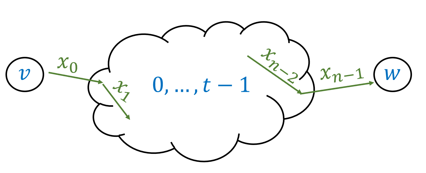
To give regular expressions for the functions \(F_{v,w}\), we start by defining the following functions \(F_{v,w}^t\): for every \(v,w \in [C]\) and \(0 \leq t \leq C\), \(F_{v,w}^t(x)=1\) if and only if starting from \(v\) and observing \(x\), the automata reaches \(w\) with all intermediate states being in the set \([t]=\{0,\ldots, t-1\}\) (see Figure 6.7). That is, while \(v,w\) themselves might be outside \([t]\), \(F_{v,w}^t(x)=1\) if and only if throughout the execution of the automaton on the input \(x\) (when initiated at \(v\)) it never enters any of the states outside \([t]\) and still ends up at \(w\). If \(t=0\) then \([t]\) is the empty set, and hence \(F^0_{v,w}(x)=1\) if and only if the automaton reaches \(w\) from \(v\) directly on \(x\), without any intermediate state. If \(t=C\) then all states are in \([t]\), and hence \(F_{v,w}^t= F_{v,w}\).
We will prove the theorem by induction on \(t\), showing that \(F^t_{v,w}\) is regular for every \(v,w\) and \(t\). For the base case of \(t=0\), \(F^0_{v,w}\) is regular for every \(v,w\) since it can be described as one of the expressions \(\ensuremath{\text{\texttt{""}}}\), \(\emptyset\), \(0\), \(1\) or \(0|1\). Specifically, if \(v=w\) then \(F^0_{v,w}(x)=1\) if and only if \(x\) is the empty string. If \(v\neq w\) then \(F^0_{v,w}(x)=1\) if and only if \(x\) consists of a single symbol \(\sigma \in \{0,1\}\) and \(T(v,\sigma)=w\). Therefore in this case \(F^0_{v,w}\) corresponds to one of the four regular expressions \(0|1\), \(0\), \(1\) or \(\emptyset\), depending on whether \(A\) transitions to \(w\) from \(v\) when it reads either \(0\) or \(1\), only one of these symbols, or neither.
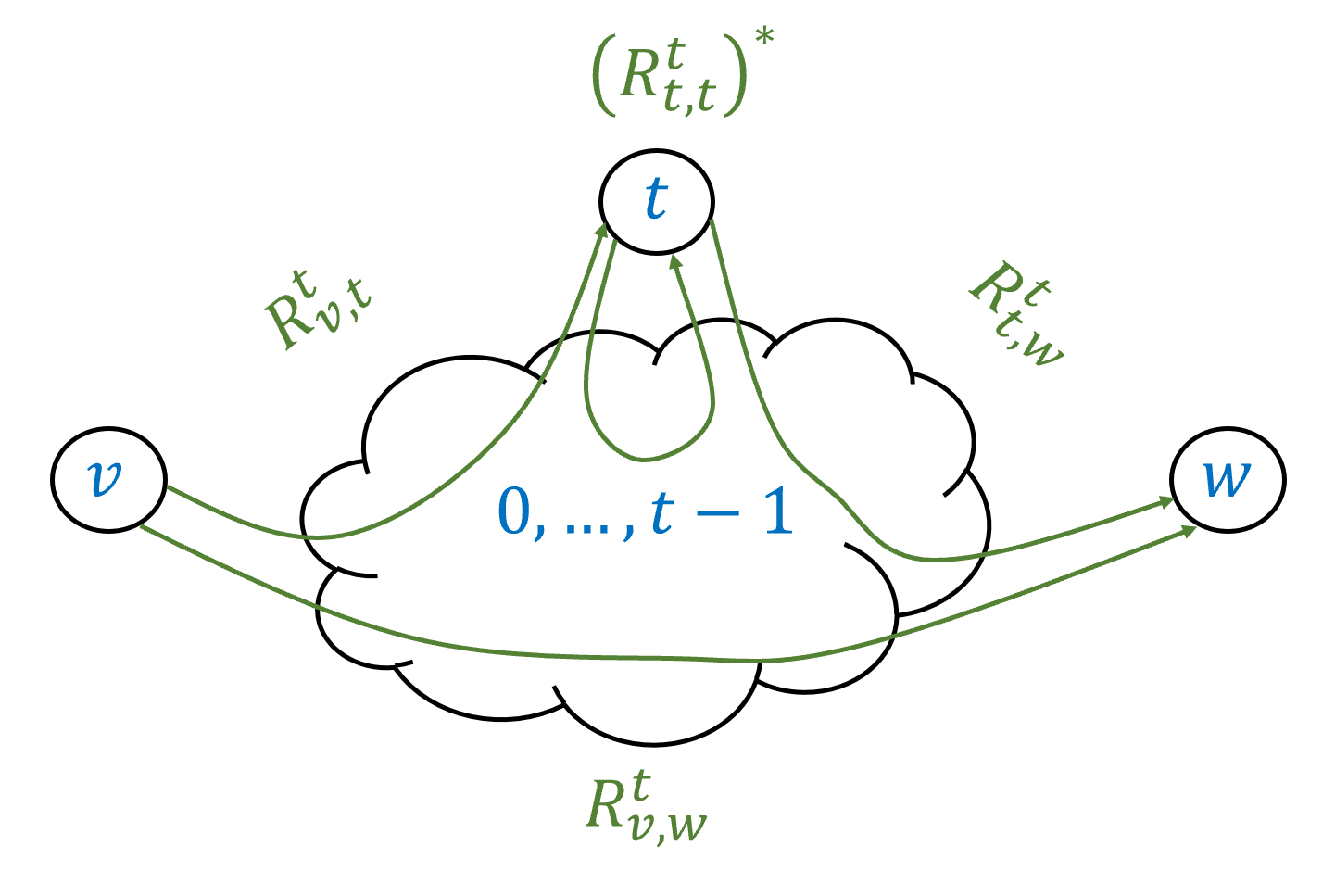
Inductive step: Now that we’ve seen the base case, let us prove the general case by induction. Assume, via the induction hypothesis, that for every \(v',w' \in [C]\), we have a regular expression \(R_{v',w'}^t\) that computes \(F_{v',w'}^t\). We need to prove that \(F_{v,w}^{t+1}\) is regular for every \(v,w\). If the automaton arrives from \(v\) to \(w\) using the intermediate states \([t+1]\), then it visits the \(t\)-th state zero or more times. If the path labeled by \(x\) causes the automaton to get from \(v\) to \(w\) without visiting the \(t\)-th state at all, then \(x\) is matched by the regular expression \(R_{v,w}^t\). If the path labeled by \(x\) causes the automaton to get from \(v\) to \(w\) while visiting the \(t\)-th state \(k>0\) times, then we can think of this path as:
First travel from \(v\) to \(t\) using only intermediate states in \([t-1]\).
Then go from \(t\) back to itself \(k-1\) times using only intermediate states in \([t-1]\)
Then go from \(t\) to \(w\) using only intermediate states in \([t-1]\).
Therefore in this case the string \(x\) is matched by the regular expression \(R_{v,t}^t(R_{t,t}^t)^* R_{t,w}^t\). (See also Figure 6.8.)
Therefore we can compute \(F_{v,w}^{t+1}\) using the regular expression
Closure properties of regular expressions
If \(F\) and \(G\) are regular functions computed by the expressions \(e\) and \(f\) respectively, then the expression \(e|f\) computes the function \(H = F \vee G\) defined as \(H(x) = F(x) \vee G(x)\). Another way to say this is that the set of regular functions is closed under the OR operation. That is, if \(F\) and \(G\) are regular then so is \(F \vee G\). An important corollary of Theorem 6.17 is that this set is also closed under the NOT operation:
If \(F:\{0,1\}^* \rightarrow \{0,1\}\) is regular then so is the function \(\overline{F}\), where \(\overline{F}(x) = 1 - F(x)\) for every \(x\in \{0,1\}^*\).
If \(F\) is regular then by Theorem 6.12 it can be computed by a DFA \(A\). But we can then construct a DFA \(\overline{A}\) which does the same computation but flips the set of accepted states. The DFA \(\overline{A}\) will compute \(\overline{F}\). By Theorem 6.17 this implies that \(\overline{F}\) is regular as well.
Since \(a \wedge b = \overline{\overline{a} \vee \overline{b}}\), Lemma 6.18 implies that the set of regular functions is closed under the AND operation as well. Moreover, since OR, NOT and AND are a universal basis, this set is also closed under NAND, XOR, and any other finite function. That is, we have the following corollary:
Let \(f:\{0,1\}^k \rightarrow \{0,1\}\) be any finite Boolean function, and let \(F_0,\ldots,F_{k-1} : \{0,1\}^* \rightarrow \{0,1\}\) be regular functions. Then the function \(G(x) = f(F_0(x),F_1(x),\ldots,F_{k-1}(x))\) is regular.
This is a direct consequence of the closure of regular functions under OR and NOT (and hence AND), combined with Theorem 4.13, that states that every \(f\) can be computed by a Boolean circuit (which is simply a combination of the AND, OR, and NOT operations).
Limitations of regular expressions and the pumping lemma
The efficiency of regular expression matching makes them very useful. This is why operating systems and text editors often restrict their search interface to regular expressions and do not allow searching by specifying an arbitrary function. However, this efficiency comes at a cost. As we have seen, regular expressions cannot compute every function. In fact, there are some very simple (and useful!) functions that they cannot compute. Here is one example:
Let \(\Sigma = \{\langle ,\rangle \}\) and \(\ensuremath{\mathit{MATCHPAREN}}:\Sigma^* \rightarrow \{0,1\}\) be the function that given a string of parentheses, outputs \(1\) if and only if every opening parenthesis is matched by a corresponding closed one. Then there is no regular expression over \(\Sigma\) that computes \(\ensuremath{\mathit{MATCHPAREN}}\).
Lemma 6.20 is a consequence of the following result, which is known as the pumping lemma:
Let \(e\) be a regular expression over some alphabet \(\Sigma\). Then there is some number \(n_0\) such that for every \(w\in \Sigma^*\) with \(|w|>n_0\) and \(\Phi_{e}(w)=1\), we can write \(w=xyz\) for strings \(x,y,z \in \Sigma^*\) satisfying the following conditions:
\(|y| \geq 1\).
\(|xy| \leq n_0\).
\(\Phi_{e}(xy^kz)=1\) for every \(k\in \N\).
The idea behind the proof is the following. Let \(n_0\) be twice the number of symbols that are used in the expression \(e\), then the only way that there is some \(w\) with \(|w|>n_0\) and \(\Phi_{e}(w)=1\) is that \(e\) contains the \(*\) (i.e. star) operator and that there is a non-empty substring \(y\) of \(w\) that was matched by \((e')^*\) for some sub-expression \(e'\) of \(e\). We can now repeat \(y\) any number of times and still get a matching string. See also Figure 6.9.
The pumping lemma is a bit cumbersome to state, but one way to remember it is that it simply says the following: “if a string matching a regular expression is long enough, one of its substrings must be matched using the \(*\) operator”.
To prove the lemma formally, we use induction on the length of the expression. Like all induction proofs, this will be somewhat lengthy, but at the end of the day it directly follows the intuition above that somewhere we must have used the star operation. Reading this proof, and in particular understanding how the formal proof below corresponds to the intuitive idea above, is a very good way to get more comfortable with inductive proofs of this form.
Our inductive hypothesis is that for an \(n\) length expression, \(n_0=2n\) satisfies the conditions of the lemma. The base case is when the expression is a single symbol \(\sigma \in \Sigma\) or that the expression is \(\emptyset\) or \(\ensuremath{\text{\texttt{""}}}\). In all these cases the conditions of the lemma are satisfied simply because \(n_0=2\), and there exists no string \(x\) of length larger than \(n_0\) that is matched by the expression.
We now prove the inductive step. Let \(e\) be a regular expression with \(n>1\) symbols. We set \(n_0=2n\) and let \(w\in \Sigma^*\) be a string satisfying \(|w|>n_0\). Since \(e\) has more than one symbol, it has one of the forms (a) \(e' | e''\), (b), \((e')(e'')\), or (c) \((e')^*\) where in all these cases the subexpressions \(e'\) and \(e''\) have fewer symbols than \(e\) and hence satisfy the induction hypothesis.
In the case (a), every string \(w\) matched by \(e\) must be matched by either \(e'\) or \(e''\). If \(e'\) matches \(w\) then, since \(|w|>2|e'|\), by the induction hypothesis there exist \(x,y,z\) with \(|y| \geq 1\) and \(|xy| \leq 2|e'| <n_0\) such that \(e'\) (and therefore also \(e=e'|e''\)) matches \(xy^kz\) for every \(k\). The same arguments works in the case that \(e''\) matches \(w\).
In the case (b), if \(w\) is matched by \((e')(e'')\) then we can write \(w=w'w''\) where \(e'\) matches \(w'\) and \(e''\) matches \(w''\). We split to subcases. If \(|w'|>2|e'|\) then by the induction hypothesis there exist \(x,y,z'\) with \(|y| \geq 1\), \(|xy| \leq 2|e'| < n_0\) such that \(w'=xyz'\) and \(e'\) matches \(xy^kz'\) for every \(k\in \N\). This completes the proof since if we set \(z=z'w''\) then we see that \(w=w'w''=xyz\) and \(e=(e')(e'')\) matches \(xy^kz\) for every \(k\in \N\). Otherwise, if \(|w'| \leq 2|e'|\) then since \(|w|=|w'|+|w''|>n_0=2(|e'|+|e''|)\), it must be that \(|w''|>2|e''|\). Hence by the induction hypothesis there exist \(x',y,z\) such that \(|y| \geq 1\), \(|x'y| \leq 2|e''|\) and \(e''\) matches \(x'y^kz\) for every \(k\in \N\). But now if we set \(x=w'x'\) we see that \(|xy| = |w'| + |x'y| \leq 2|e'| + 2|e''| =n_0\) and on the other hand the expression \(e=(e')(e'')\) matches \(xy^kz = w'x'y^kz\) for every \(k\in \N\).
In case (c), if \(w\) is matched by \((e')^*\) then \(w= w_0\cdots w_t\) where for every \(i\in [t]\), \(w_i\) is a nonempty string matched by \(e'\). If \(|w_0|>2|e'|\), then we can use the same approach as in the concatenation case above. Otherwise, we simply note that if \(x\) is the empty string, \(y=w_0\), and \(z=w_1\cdots w_t\) then \(|xy| \leq n_0\) and \(xy^kz\) is matched by \((e')^*\) for every \(k\in \N\).
When an object is recursively defined (as in the case of regular expressions) then it is natural to prove properties of such objects by induction. That is, if we want to prove that all objects of this type have property \(P\), then it is natural to use an inductive step that says that if \(o',o'',o'''\) etc have property \(P\) then so is an object \(o\) that is obtained by composing them.
Using the pumping lemma, we can easily prove Lemma 6.20 (i.e., the non-regularity of the “matching parenthesis” function):
Suppose, towards the sake of contradiction, that there is an expression \(e\) such that \(\Phi_{e}= \ensuremath{\mathit{MATCHPAREN}}\). Let \(n_0\) be the number obtained from Theorem 6.21 and let \(w =\langle^{n_0}\rangle^{n_0}\) (i.e., \(n_0\) left parenthesis followed by \(n_0\) right parenthesis). Then we see that if we write \(w=xyz\) as in Theorem 6.21, the condition \(|xy| \leq n_0\) implies that \(y\) consists solely of left parenthesis. Hence the string \(xy^2z\) will contain more left parenthesis than right parenthesis. Hence \(\ensuremath{\mathit{MATCHPAREN}}(xy^2z)=0\) but by the pumping lemma \(\Phi_{e}(xy^2z)=1\), contradicting our assumption that \(\Phi_{e}=\ensuremath{\mathit{MATCHPAREN}}\).
The pumping lemma is a very useful tool to show that certain functions are not computable by a regular expression. However, it is not an “if and only if” condition for regularity: there are non-regular functions that still satisfy the pumping lemma conditions. To understand the pumping lemma, it is crucial to follow the order of quantifiers in Theorem 6.21. In particular, the number \(n_0\) in the statement of Theorem 6.21 depends on the regular expression (in the proof we chose \(n_0\) to be twice the number of symbols in the expression). So, if we want to use the pumping lemma to rule out the existence of a regular expression \(e\) computing some function \(F\), we need to be able to choose an appropriate input \(w\in \{0,1\}^*\) that can be arbitrarily large and satisfies \(F(w)=1\). This makes sense if you think about the intuition behind the pumping lemma: we need \(w\) to be large enough as to force the use of the star operator.
Prove that the following function over the alphabet \(\{0,1,; \}\) is not regular: \(\ensuremath{\mathit{PAL}}(w)=1\) if and only if \(w = u;u^R\) where \(u \in \{0,1\}^*\) and \(u^R\) denotes \(u\) “reversed”: the string \(u_{|u|-1}\cdots u_0\). (The Palindrome function is most often defined without an explicit separator character \(;\), but the version with such a separator is a bit cleaner, and so we use it here. This does not make much difference, as one can easily encode the separator as a special binary string instead.)
We use the pumping lemma. Suppose toward the sake of contradiction that there is a regular expression \(e\) computing \(\ensuremath{\mathit{PAL}}\), and let \(n_0\) be the number obtained by the pumping lemma (Theorem 6.21). Consider the string \(w = 0^{n_0};0^{n_0}\). Since the reverse of the all zero string is the all zero string, \(\ensuremath{\mathit{PAL}}(w)=1\). Now, by the pumping lemma, if \(\ensuremath{\mathit{PAL}}\) is computed by \(e\), then we can write \(w=xyz\) such that \(|xy| \leq n_0\), \(|y|\geq 1\) and \(\ensuremath{\mathit{PAL}}(xy^kz)=1\) for every \(k\in \N\). In particular, it must hold that \(\ensuremath{\mathit{PAL}}(xz)=1\), but this is a contradiction, since \(xz=0^{n_0-|y|};0^{n_0}\) and so its two parts are not of the same length and in particular are not the reverse of one another.
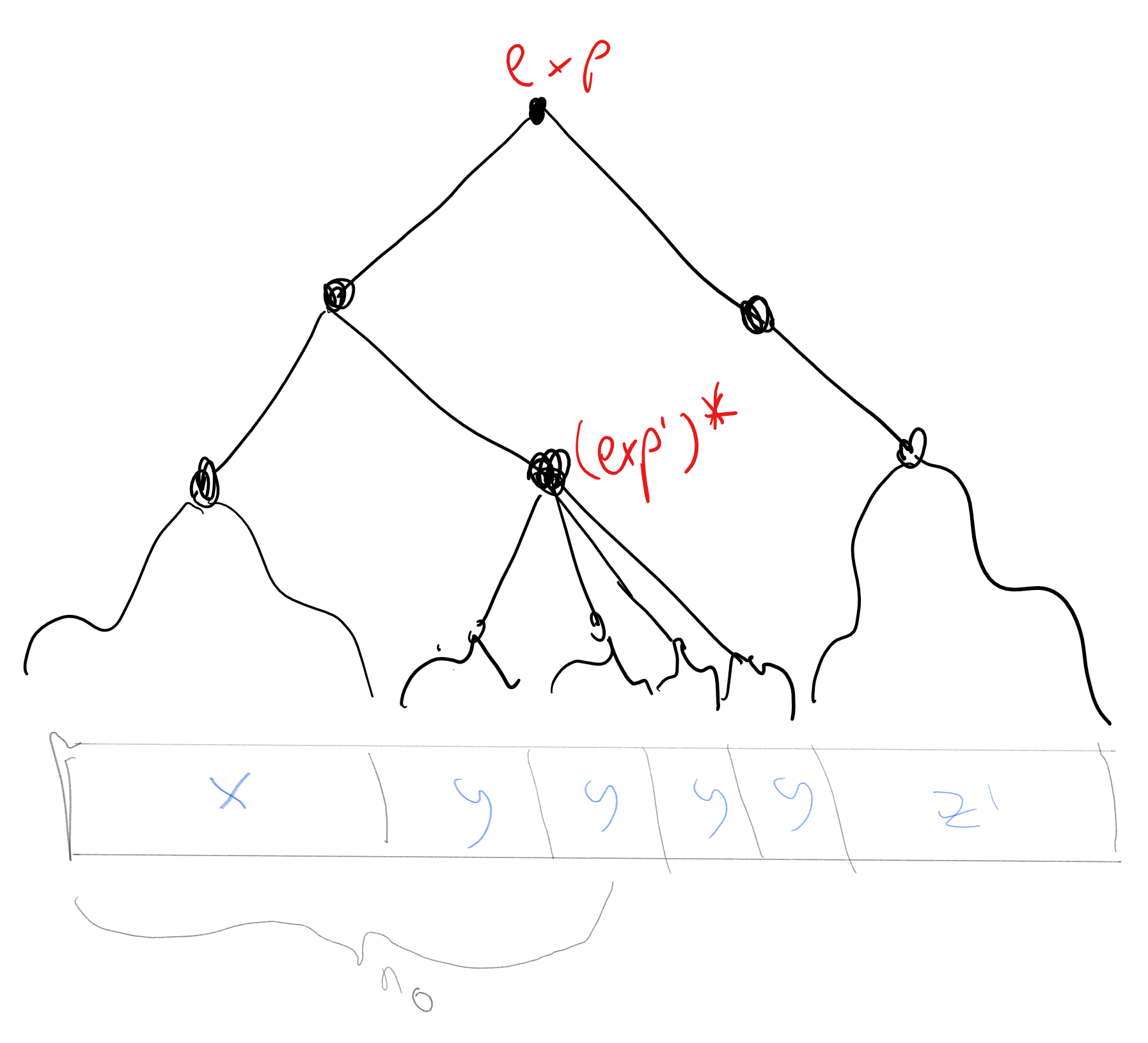
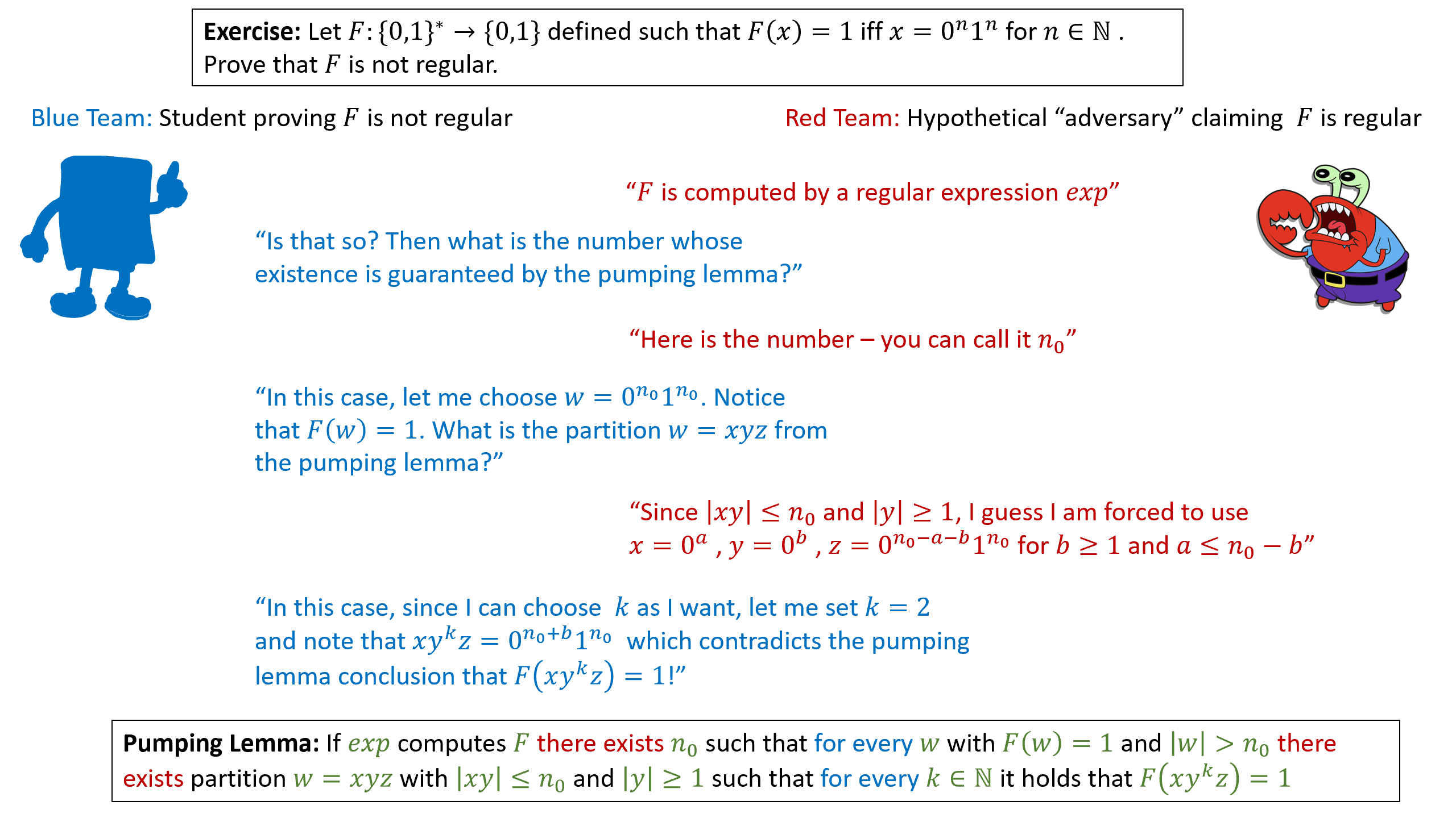
For yet another example of a pumping-lemma based proof, see Figure 6.10 which illustrates a cartoon of the proof of the non-regularity of the function \(F:\{0,1\}^* \rightarrow \{0,1\}\) which is defined as \(F(x)=1\) iff \(x=0^n1^n\) for some \(n\in \N\) (i.e., \(x\) consists of a string of consecutive zeroes, followed by a string of consecutive ones of the same length).
Answering semantic questions about regular expressions
Regular expressions have applications beyond search. For example, regular expressions are often used to define tokens (such as what is a valid variable identifier, or keyword) in the design of parsers, compilers and interpreters for programming languages. Regular expressions have other applications too: for example, in recent years, the world of networking moved from fixed topologies to “software defined networks”. Such networks are routed by programmable switches that can implement policies such as “if packet is secured by SSL then forward it to A, otherwise forward it to B”. To represent such policies we need a language that is on one hand sufficiently expressive to capture the policies we want to implement, but on the other hand sufficiently restrictive so that we can quickly execute them at network speed and also be able to answer questions such as “can C see the packets moved from A to B?”. The NetKAT network programming language uses a variant of regular expressions to achieve precisely that. For this application, it is important that we are not merely able to answer whether an expression \(e\) matches a string \(x\) but also answer semantic questions about regular expressions such as “do expressions \(e\) and \(e'\) compute the same function?” and “does there exist a string \(x\) that is matched by the expression \(e\)?”. The following theorem shows that we can answer the latter question:
There is an algorithm that given a regular expression \(e\), outputs \(1\) if and only if \(\Phi_{e}\) is the constant zero function.
The idea is that we can directly observe this from the structure of the expression. The only way a regular expression \(e\) computes the constant zero function is if \(e\) has the form \(\emptyset\) or is obtained by concatenating \(\emptyset\) with other expressions.
Define a regular expression to be “empty” if it computes the constant zero function. Given a regular expression \(e\), we can determine if \(e\) is empty using the following rules:
If \(e\) has the form \(\sigma\) or \(\ensuremath{\text{\texttt{""}}}\) then it is not empty.
If \(e\) is not empty then \(e|e'\) is not empty for every \(e'\).
If \(e\) is not empty then \(e^*\) is not empty.
If \(e\) and \(e'\) are both not empty then \(e\; e'\) is not empty.
\(\emptyset\) is empty.
Using these rules, it is straightforward to come up with a recursive algorithm to determine emptiness.
Using Theorem 6.23, we can obtain an algorithm that determines whether or not two regular expressions \(e\) and \(e'\) are equivalent, in the sense that they compute the same function.
Let \(\ensuremath{\mathit{REGEQ}}:\{0,1\}^* \rightarrow \{0,1\}\) be the function that on input (a string representing) a pair of regular expressions \(e,e'\), \(\ensuremath{\mathit{REGEQ}}(e,e')=1\) if and only if \(\Phi_{e} = \Phi_{e'}\). Then there is an algorithm that computes \(\ensuremath{\mathit{REGEQ}}\).
The idea is to show that given a pair of regular expressions \(e\) and \(e'\) we can find an expression \(e''\) such that \(\Phi_{e''}(x)=1\) if and only if \(\Phi_e(x) \neq \Phi_{e'} (x)\). Therefore \(\Phi_{e''}\) is the constant zero function if and only if \(e\) and \(e'\) are equivalent, and thus we can test for emptiness of \(e''\) to determine equivalence of \(e\) and \(e'\).
We will prove Theorem 6.24 from Theorem 6.23. (The two theorems are in fact equivalent: it is easy to prove Theorem 6.23 from Theorem 6.24, since checking for emptiness is the same as checking equivalence with the expression \(\emptyset\).) Given two regular expressions \(e\) and \(e'\), we will compute an expression \(e''\) such that \(\Phi_{e''}(x) =1\) if and only if \(\Phi_e(x) \neq \Phi_{e'}(x)\). One can see that \(e\) is equivalent to \(e'\) if and only if \(e''\) is empty.
We start with the observation that for every bit \(a,b \in \{0,1\}\), \(a \neq b\) if and only if
Hence we need to construct \(e''\) such that for every \(x\),
To construct the expression \(e''\), we will show how given any pair of expressions \(e\) and \(e'\), we can construct expressions \(e\wedge e'\) and \(\overline{e}\) that compute the functions \(\Phi_{e} \wedge \Phi_{e'}\) and \(\overline{\Phi_{e}}\) respectively. (Computing the expression for \(e \vee e'\) is straightforward using the \(|\) operation of regular expressions.)
Specifically, by Lemma 6.18, regular functions are closed under negation, which means that for every regular expression \(e\), there is an expression \(\overline{e}\) such that \(\Phi_{\overline{e}}(x) = 1 - \Phi_{e}(x)\) for every \(x\in \{0,1\}^*\). Now, for every two expressions \(e\) and \(e'\), the expression
- We model computational tasks on arbitrarily large inputs using infinite functions \(F:\{0,1\}^* \rightarrow \{0,1\}^*\).
- Such functions take an arbitrarily long (but still finite!) string as input, and cannot be described by a finite table of inputs and outputs.
- A function with a single bit of output is known as a Boolean function, and the task of computing it is equivalent to deciding a language \(L\subseteq \{0,1\}^*\).
- Deterministic finite automata (DFAs) are one simple model for computing (infinite) Boolean functions.
- There are some functions that cannot be computed by DFAs.
- The set of functions computable by DFAs is the same as the set of languages that can be recognized by regular expressions.
Exercises
Suppose that \(F,G:\{0,1\}^* \rightarrow \{0,1\}\) are regular. For each one of the following definitions of the function \(H\), either prove that \(H\) is always regular or give a counterexample for regular \(F,G\) that would make \(H\) not regular.
\(H(x) = F(x) \vee G(x)\).
\(H(x) = F(x) \wedge G(x)\)
\(H(x) = \ensuremath{\mathit{NAND}}(F(x),G(x))\).
\(H(x) = F(x^R)\) where \(x^R\) is the reverse of \(x\): \(x^R = x_{n-1}x_{n-2} \cdots x_o\) for \(n=|x|\).
\(H(x) = \begin{cases}1 & x=uv \text{ s.t. } F(u)=G(v)=1 \\ 0 & \text{otherwise} \end{cases}\)
\(H(x) = \begin{cases}1 & x=uu \text{ s.t. } F(u)=G(u)=1 \\ 0 & \text{otherwise} \end{cases}\)
\(H(x) = \begin{cases}1 & x=uu^R \text{ s.t. } F(u)=G(u)=1 \\ 0 & \text{otherwise} \end{cases}\)
One among the following two functions that map \(\{0,1\}^*\) to \(\{0,1\}\) can be computed by a regular expression, and the other one cannot. For the one that can be computed by a regular expression, write the expression that does it. For the one that cannot, prove that this cannot be done using the pumping lemma.
\(F(x)=1\) if \(4\) divides \(\sum_{i=0}^{|x|-1} x_i\) and \(F(x)=0\) otherwise.
\(G(x) = 1\) if and only if \(\sum_{i=0}^{|x|-1} x_i \geq |x|/4\) and \(G(x)=0\) otherwise.
Prove that the following function \(F:\{0,1\}^* \rightarrow \{0,1\}\) is not regular. For every \(x\in \{0,1\}^*\), \(F(x)=1\) iff \(x\) is of the form \(x=1^{3^i}\) for some \(i>0\).
Prove that the following function \(F:\{0,1\}^* \rightarrow \{0,1\}\) is not regular. For every \(x\in \{0,1\}^*\), \(F(x)=1\) iff \(\sum_j x_j = 3^i\) for some \(i>0\).
Bibliographical notes
The relation of regular expressions with finite automata is a beautiful topic, on which we only touch upon in this text. It is covered more extensively in (Sipser, 1997) (Hopcroft, Motwani, Ullman, 2014) (Kozen, 1997) . These texts also discuss topics such as non-deterministic finite automata (NFA) and the relation between context-free grammars and pushdown automata.
The automaton of Figure 6.4 was generated using the FSM simulator of Ivan Zuzak and Vedrana Jankovic. Our proof of Theorem 6.12 is closely related to the Myhill-Nerode Theorem. One direction of the Myhill-Nerode theorem can be stated as saying that if \(e\) is a regular expression then there is at most a finite number of strings \(z_0,\ldots,z_{k-1}\) such that \(\Phi_{e[z_i]} \neq \Phi_{e[z_j]}\) for every \(0 \leq i\neq j < k\).
Comments
Comments are posted on the GitHub repository using the utteranc.es app. A GitHub login is required to comment. If you don't want to authorize the app to post on your behalf, you can also comment directly on the GitHub issue for this page.
Compiled on 12/06/2023 00:07:03
Copyright 2023, Boaz Barak.

This work is
licensed under a Creative Commons
Attribution-NonCommercial-NoDerivatives 4.0 International License.
Produced using pandoc and panflute with templates derived from gitbook and bookdown.