See any bugs/typos/confusing explanations? Open a GitHub issue. You can also comment below
★ See also the PDF version of this chapter (better formatting/references) ★
Computation and Representation
- Distinguish between specification and implementation, or equivalently between mathematical functions and algorithms/programs.
- Representing an object as a string (often of zeroes and ones).
- Examples of representations for common objects such as numbers, vectors, lists, and graphs.
- Prefix-free representations.
- Cantor’s Theorem: The real numbers cannot be represented exactly as finite strings.
“The alphabet (sic) was a great invention, which enabled men (sic) to store and to learn with little effort what others had learned the hard way – that is, to learn from books rather than from direct, possibly painful, contact with the real world.”, B.F. Skinner
“The name of the song is called `HADDOCK’S EYES.’” [said the Knight]
“Oh, that’s the name of the song, is it?” Alice said, trying to feel interested.
“No, you don’t understand,” the Knight said, looking a little vexed. “That’s what the name is CALLED. The name really is `THE AGED AGED MAN.’”
“Then I ought to have said `That’s what the SONG is called’?” Alice corrected herself.
“No, you oughtn’t: that’s quite another thing! The SONG is called `WAYS AND MEANS’: but that’s only what it’s CALLED, you know!”
“Well, what IS the song, then?” said Alice, who was by this time completely bewildered.
“I was coming to that,” the Knight said. “The song really IS `A-SITTING ON A GATE’: and the tune’s my own invention.”
Lewis Carroll, Through the Looking-Glass
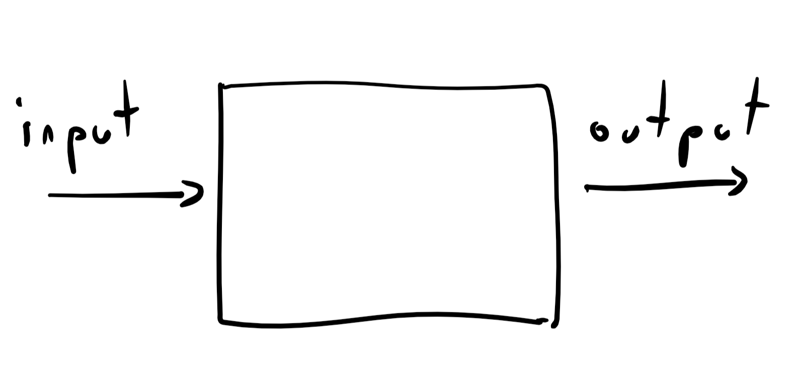
To a first approximation, computation is a process that maps an input to an output.
When discussing computation, it is essential to separate the question of what is the task we need to perform (i.e., the specification) from the question of how we achieve this task (i.e., the implementation). For example, as we’ve seen, there is more than one way to achieve the computational task of computing the product of two integers.
In this chapter we focus on the what part, namely defining computational tasks. For starters, we need to define the inputs and outputs. Capturing all the potential inputs and outputs that we might ever want to compute seems challenging, since computation today is applied to a wide variety of objects. We do not compute merely on numbers, but also on texts, images, videos, connection graphs of social networks, MRI scans, gene data, and even other programs. We will represent all these objects as strings of zeroes and ones, that is objects such as \(0011101\) or \(1011\) or any other finite list of \(1\)’s and \(0\)’s. (This choice is for convenience: there is nothing “holy” about zeroes and ones, and we could have used any other finite collection of symbols.)
Today, we are so used to the notion of digital representation that we are not surprised by the existence of such an encoding. But it is actually a deep insight with significant implications. Many animals can convey a particular fear or desire, but what is unique about humans is language: we use a finite collection of basic symbols to describe a potentially unlimited range of experiences. Language allows transmission of information over both time and space and enables societies that span a great many people and accumulate a body of shared knowledge over time.
Over the last several decades, we have seen a revolution in what we can represent and convey in digital form. We can capture experiences with almost perfect fidelity, and disseminate it essentially instantaneously to an unlimited audience. Moreover, once information is in digital form, we can compute over it, and gain insights from data that were not accessible in prior times. At the heart of this revolution is the simple but profound observation that we can represent an unbounded variety of objects using a finite set of symbols (and in fact using only the two symbols 0 and 1).
In later chapters, we will typically take such representations for granted, and hence use expressions such as “program \(P\) takes \(x\) as input” when \(x\) might be a number, a vector, a graph, or any other object, when we really mean that \(P\) takes as input the representation of \(x\) as a binary string. However, in this chapter we will dwell a bit more on how we can construct such representations.
The main takeaways from this chapter are:
We can represent all kinds of objects we want to use as inputs and outputs using binary strings. For example, we can use the binary basis to represent integers and rational numbers as binary strings (see Section 2.1.1 and Section 2.2).
We can compose the representations of simple objects to represent more complex objects. In this way, we can represent lists of integers or rational numbers, and use that to represent objects such as matrices, images, and graphs. Prefix-free encoding is one way to achieve such a composition (see Section 2.5.2).
A computational task specifies a map from an input to an output— a function. It is crucially important to distinguish between the “what” and the “how”, or the specification and implementation (see Section 2.6.1). A function simply defines which output corresponds to which input. It does not specify how to compute the output from the input, and as we’ve seen in the context of multiplication, there can be more than one way to compute the same function.
While the set of all possible binary strings is infinite, it still cannot represent everything. In particular, there is no representation of the real numbers (with absolute accuracy) as binary strings. This result is also known as “Cantor’s Theorem” (see Section 2.4) and is typically referred to as the result that the “reals are uncountable.” It is also implied that there are different levels of infinity though we will not get into this topic in this book (see Remark 2.10).
The two “big ideas” we discuss are Big Idea 1 - we can compose representations for simple objects to represent more complex objects and Big Idea 2 - it is crucial to distinguish between functions’ (“what”) and programs’ (“how”). The latter will be a theme we will come back to time and again in this book.
Defining representations
Every time we store numbers, images, sounds, databases, or other objects on a computer, what we actually store in the computer’s memory is the representation of these objects. Moreover, the idea of representation is not restricted to digital computers. When we write down text or make a drawing we are representing ideas or experiences as sequences of symbols (which might as well be strings of zeroes and ones). Even our brain does not store the actual sensory inputs we experience, but rather only a representation of them.
To use objects such as numbers, images, graphs, or others as inputs for computation, we need to define precisely how to represent these objects as binary strings. A representation scheme is a way to map an object \(x\) to a binary string \(E(x) \in \{0,1\}^*\). For example, a representation scheme for natural numbers is a function \(E:\N \rightarrow \{0,1\}^*\). Of course, we cannot merely represent all numbers as the string “\(0011\)” (for example). A minimal requirement is that if two numbers \(x\) and \(x'\) are different then they would be represented by different strings. Another way to say this is that we require the encoding function \(E\) to be one to one.
Representing natural numbers
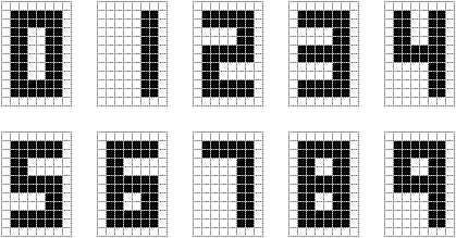
We now show how we can represent natural numbers as binary strings. Over the years people have represented numbers in a variety of ways, including Roman numerals, tally marks, our own Hindu-Arabic decimal system, and many others. We can use any one of those as well as many others to represent a number as a string (see Figure 2.3). However, for the sake of concreteness, we use the binary basis as our default representation of natural numbers as strings. For example, we represent the number six as the string \(110\) since \(1\cdot 2^{2} + 1 \cdot 2^1 + 0 \cdot 2^0 = 6\), and similarly we represent the number thirty-five as the string \(y = 100011\) which satisfies \(\sum_{i=0}^5 y_i \cdot 2^{|y|-i-1} = 35\). Some more examples are given in the table below.
| Number (decimal representation) | Number (binary representation) |
|---|---|
| 0 | 0 |
| 1 | 1 |
| 2 | 10 |
| 5 | 101 |
| 16 | 10000 |
| 40 | 101000 |
| 53 | 110101 |
| 389 | 110000101 |
| 3750 | 111010100110 |
If \(n\) is even, then the least significant digit of \(n\)’s binary representation is \(0\), while if \(n\) is odd then this digit equals \(1\). Just like the number \(\floor{n/10}\) corresponds to “chopping off” the least significant decimal digit (e.g., \(\floor{457/10}=\floor{45.7}=45\)), the number \(\floor{n/2}\) corresponds to the “chopping off” the least significant binary digit. Hence the binary representation can be formally defined as the following function \(NtS:\N \rightarrow \{0,1\}^*\) (\(NtS\) stands for “natural numbers to strings”):
where \(parity:\N \rightarrow \{0,1\}\) is the function defined as \(parity(n)=0\) if \(n\) is even and \(parity(n)=1\) if \(n\) is odd, and as usual, for strings \(x,y \in \{0,1\}^*\), \(xy\) denotes the concatenation of \(x\) and \(y\). The function \(NtS\) is defined recursively: for every \(n>1\) we define \(rep(n)\) in terms of the representation of the smaller number \(\floor{n/2}\). It is also possible to define \(NtS\) non-recursively, see Exercise 2.2.
Throughout most of this book, the particular choices of representation of numbers as binary strings would not matter much: we just need to know that such a representation exists. In fact, for many of our purposes we can even use the simpler representation of mapping a natural number \(n\) to the length-\(n\) all-zero string \(0^n\).
We can implement the binary representation in Python as follows:
def NtS(n):# natural numbers to strings
    if n > 1:
        return NtS(n // 2) + str(n % 2)
    else:
        return str(n % 2)

print(NtS(236))
# 11101100

print(NtS(19))
# 10011
We can also use Python to implement the inverse transformation, mapping a string back to the natural number it represents.
In this book, we sometimes use code examples as in Remark 2.1. The point is always to emphasize that certain computations can be achieved concretely, rather than illustrating the features of Python or any other programming language. Indeed, one of the messages of this book is that all programming languages are in a certain precise sense equivalent to one another, and hence we could have just as well used JavaScript, C, COBOL, Visual Basic or even BrainF*ck. This book is not about programming, and it is absolutely OK if you are not familiar with Python or do not follow code examples such as those in Remark 2.1.
Meaning of representations (discussion)
It is natural for us to think of \(236\) as the “actual” number, and of \(11101100\) as “merely” its representation. However, for most Europeans in the middle ages CCXXXVI would be the “actual” number and \(236\) (if they have even heard about it) would be the weird Hindu-Arabic positional representation.1 When our AI robot overlords materialize, they will probably think of \(11101100\) as the “actual” number and of \(236\) as “merely” a representation that they need to use when they give commands to humans.
So what is the “actual” number? This is a question that philosophers of mathematics have pondered throughout history. Plato argued that mathematical objects exist in some ideal sphere of existence (that to a certain extent is more “real” than the world we perceive via our senses, as this latter world is merely the shadow of this ideal sphere). In Plato’s vision, the symbols \(236\) are merely notation for some ideal object, that, in homage to the late musician, we can refer to as “the number commonly represented by \(236\)”.
The Austrian philosopher Ludwig Wittgenstein, on the other hand, argued that mathematical objects do not exist at all, and the only things that exist are the actual marks on paper that make up \(236\), \(11101100\) or CCXXXVI. In Wittgenstein’s view, mathematics is merely about formal manipulation of symbols that do not have any inherent meaning. You can think of the “actual” number as (somewhat recursively) “that thing which is common to \(236\), \(11101100\) and CCXXXVI and all other past and future representations that are meant to capture the same object”.
While reading this book, you are free to choose your own philosophy of mathematics, as long as you maintain the distinction between the mathematical objects themselves and the various particular choices of representing them, whether as splotches of ink, pixels on a screen, zeroes and ones, or any other form.
Representations beyond natural numbers
We have seen that natural numbers can be represented as binary strings. We now show that the same is true for other types of objects, including (potentially negative) integers, rational numbers, vectors, lists, graphs and many others. In many instances, choosing the “right” string representation for a piece of data is highly non-trivial, and finding the “best” one (e.g., most compact, best fidelity, most efficiently manipulable, robust to errors, most informative features, etc.) is the object of intense research. But for now, we focus on presenting some simple representations for various objects that we would like to use as inputs and outputs for computation.
Representing (potentially negative) integers
Since we can represent natural numbers as strings, we can represent the full set of integers (i.e., members of the set \(\Z=\{ \ldots, -3 , -2 , -1 , 0 , +1, +2, +3,\ldots \}\) ) by adding one more bit that represents the sign. To represent a (potentially negative) number \(m\), we prepend to the representation of the natural number \(|m|\) a bit \(\sigma\) that equals \(0\) if \(m \geq 0\) and equals \(1\) if \(m<0\). Formally, we define the function \(ZtS:\Z \rightarrow \{0,1\}^*\) as follows
While the encoding function of a representation needs to be one to one, it does not have to be onto. For example, in the representation above there is no number that is represented by the empty string but it is still a fine representation, since every integer is represented uniquely by some string.
Given a string \(y\in \{0,1\}^*\), how do we know if it’s “supposed” to represent a (non-negative) natural number or a (potentially negative) integer? For that matter, even if we know \(y\) is “supposed” to be an integer, how do we know what representation scheme it uses? The short answer is that we do not necessarily know this information, unless it is supplied from the context. (In programming languages, the compiler or interpreter determines the representation of the sequence of bits corresponding to a variable based on the variable’s type.) We can treat the same string \(y\) as representing a natural number, an integer, a piece of text, an image, or a green gremlin. Whenever we say a sentence such as “let \(n\) be the number represented by the string \(y\),” we will assume that we are fixing some canonical representation scheme such as the ones above. The choice of the particular representation scheme will rarely matter, except that we want to make sure to stick with the same one for consistency.
Two’s complement representation (optional)
Section 2.2.1’s approach of representing an integer using a specific “sign bit” is known as the Signed Magnitude Representation and was used in some early computers. However, the two’s complement representation is much more common in practice. The two’s complement representation of an integer \(k\) in the set \(\{ -2^n , -2^n+1, \ldots, 2^n-1 \}\) is the string \(ZtS_n(k)\) of length \(n+1\) defined as follows:
Another way to say this is that we represent a potentially negative number \(k \in \{ -2^n,\ldots, 2^n-1 \}\) as the non-negative number \(k \mod 2^{n+1}\) (see also Figure 2.4). This means that if two (potentially negative) numbers \(k\) and \(k'\) are not too large (i.e., $ k + k’ { -2^n,, 2^n-1 }$), then we can compute the representation of \(k+k'\) by adding modulo \(2^{n+1}\) the representations of \(k\) and \(k'\) as if they were non-negative integers. This property of the two’s complement representation is its main attraction since, depending on their architectures, microprocessors can often perform arithmetic operations modulo \(2^w\) very efficiently (for certain values of \(w\) such as \(32\) and \(64\)). Many systems leave it to the programmer to check that values are not too large and will carry out this modular arithmetic regardless of the size of the numbers involved. For this reason, in some systems adding two large positive numbers can result in a negative number (e.g., adding \(2^n-100\) and \(2^n-200\) might result in \(-300\) since \((2^{n+1}-300) \mod 2^{n+1} = -300\), see also Figure 2.4).
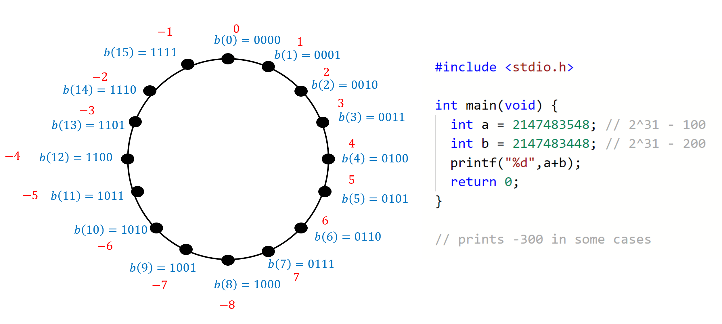
C program that will on some \(32\) bit architecture print a negative number after adding two positive numbers. (Integer overflow in C is considered undefined behavior which means the result of this program, including whether it runs or crashes, could differ depending on the architecture, compiler, and even compiler options and version.)Rational numbers and representing pairs of strings
We can represent a rational number of the form \(a/b\) by representing the two numbers \(a\) and \(b\). However, merely concatenating the representations of \(a\) and \(b\) will not work. For example, the binary representation of \(4\) is \(100\) and the binary representation of \(43\) is \(101011\), but the concatenation \(100101011\) of these strings is also the concatenation of the representation \(10010\) of \(18\) and the representation \(1011\) of \(11\). Hence, if we used such simple concatenation then we would not be able to tell if the string \(100101011\) is supposed to represent \(4/43\) or \(18/11\).
We tackle this by giving a general representation for pairs of strings. If we were using a pen and paper, we would just use a separator symbol such as \(\|\) to represent, for example, the pair consisting of the numbers represented by \(10\) and \(110001\) as the length-\(9\) string “\(10\|110001\)”. In other words, there is a one to one map \(F\) from pairs of strings \(x,y \in \{0,1\}^*\) into a single string \(z\) over the alphabet \(\Sigma = \{0,1,\| \}\) (in other words, \(z\in \Sigma^*\)). Using such separators is similar to the way we use spaces and punctuation to separate words in English. By adding a little redundancy, we achieve the same effect in the digital domain. We can map the three-element set \(\Sigma\) to the three-element set \(\{00,11,01 \} \subset \{0,1\}^2\) in a one-to-one fashion, and hence encode a length \(n\) string \(z\in \Sigma^*\) as a length \(2n\) string \(w\in \{0,1\}^*\).
Our final representation for rational numbers is obtained by composing the following steps:
Representing a (potentially negative) rational number as a pair of integers \(a,b\) such that \(r=a/b\).
Representing an integer by a string via the binary representation.
Combining 1 and 2 to obtain a representation of a rational number as a pair of strings.
Representing a pair of strings over \(\{0,1\}\) as a single string over \(\Sigma = \{0,1,\|\}\).
Representing a string over \(\Sigma\) as a longer string over \(\{0,1\}\).
Consider the rational number \(r=-5/8\). We represent \(-5\) as \(1101\) and \(+8\) as \(01000\), and so we can represent \(r\) as the pair of strings \((1101,01000)\) and represent this pair as the length \(10\) string \(1101\|01000\) over the alphabet \(\{0,1,\|\}\). Now, applying the map \(0 \mapsto 00\), \(1\mapsto 11\), \(\| \mapsto 01\), we can represent the latter string as the length \(20\) string \(s=11110011010011000000\) over the alphabet \(\{0,1\}\).
The same idea can be used to represent triples of strings, quadruples, and so on as a string. Indeed, this is one instance of a very general principle that we use time and again in both the theory and practice of computer science (for example, in Object Oriented programming):
If we can represent objects of type \(T\) as strings, then we can represent tuples of objects of type \(T\) as strings as well.
Repeating the same idea, once we can represent objects of type \(T\), we can also represent lists of lists of such objects, and even lists of lists of lists and so on and so forth. We will come back to this point when we discuss prefix free encoding in Section 2.5.2.
Representing real numbers
The set of real numbers \(\R\) contains all numbers including positive, negative, and fractional, as well as irrational numbers such as \(\pi\) or \(e\). Every real number can be approximated by a rational number, and thus we can represent every real number \(x\) by a rational number \(a/b\) that is very close to \(x\). For example, we can represent \(\pi\) by \(22/7\) within an error of about \(10^{-3}\). If we want a smaller error (e.g., about \(10^{-4}\)) then we can use \(311/99\), and so on and so forth.
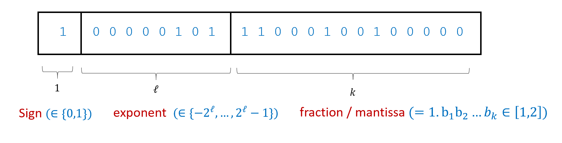
The above representation of real numbers via rational numbers that approximate them is a fine choice for a representation scheme. However, typically in computing applications, it is more common to use the floating-point representation scheme (see Figure 2.5) to represent real numbers. In the floating-point representation scheme we represent \(x\in \R\) by the pair \((b,e)\) of (positive or negative) integers of some prescribed sizes (determined by the desired accuracy) such that \(b \times 2^{e}\) is closest to \(x\). Floating-point representation is the base-two version of scientific notation, where one represents a number \(y\in R\) as its approximation of the form \(b \times 10^e\) for \(b,e\). It is called “floating-point” because we can think of the number \(b\) as specifying a sequence of binary digits, and \(e\) as describing the location of the “binary point” within this sequence. The use of floating representation is the reason why in many programming systems, printing the expression 0.1+0.2 will result in 0.30000000000000004 and not 0.3, see here, here and here for more.
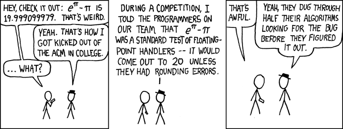
The reader might be (rightly) worried about the fact that the floating-point representation (or the rational number one) can only approximately represent real numbers. In many (though not all) computational applications, one can make the accuracy tight enough so that this does not affect the final result, though sometimes we do need to be careful. Indeed, floating-point bugs can sometimes be no joking matter. For example, floating-point rounding errors have been implicated in the failure of a U.S. Patriot missile to intercept an Iraqi Scud missile, costing 28 lives, as well as a 100 million pound error in computing payouts to British pensioners.
Cantor’s Theorem, countable sets, and string representations of the real numbers
“For any collection of fruits, we can make more fruit salads than there are fruits. If not, we could label each salad with a different fruit, and consider the salad of all fruits not in their salad. The label of this salad is in it if and only if it is not.”, Martha Storey.
Given the issues with floating-point approximations for real numbers, a natural question is whether it is possible to represent real numbers exactly as strings. Unfortunately, the following theorem shows that this cannot be done:
There does not exist a one-to-one function \(RtS:\R \rightarrow \{0,1\}^*\).2
Countable sets. We say that a set \(S\) is countable if there is an onto map \(C:\N \rightarrow S\), or in other words, we can write \(S\) as the sequence \(C(0),C(1),C(2),\ldots\). Since the binary representation yields an onto map from \(\{0,1\}^*\) to \(\N\), and the composition of two onto maps is onto, a set \(S\) is countable iff there is an onto map from \(\{0,1\}^*\) to \(S\). Using the basic properties of functions (see Section 1.4.3), a set is countable if and only if there is a one-to-one function from \(S\) to \(\{0,1\}^*\). Hence, we can rephrase Theorem 2.5 as follows:
The reals are uncountable. That is, there does not exist an onto function \(NtR:\N \rightarrow \R\).
Theorem 2.6 was proven by Georg Cantor in 1874. This result (and the theory around it) was quite shocking to mathematicians at the time. By showing that there is no one-to-one map from \(\R\) to \(\{0,1\}^*\) (or \(\N\)), Cantor showed that these two infinite sets have “different forms of infinity” and that the set of real numbers \(\R\) is in some sense “bigger” than the infinite set \(\{0,1\}^*\). The notion that there are “shades of infinity” was deeply disturbing to mathematicians and philosophers at the time. The philosopher Ludwig Wittgenstein (whom we mentioned before) called Cantor’s results “utter nonsense” and “laughable.” Others thought they were even worse than that. Leopold Kronecker called Cantor a “corrupter of youth,” while Henri Poincaré said that Cantor’s ideas “should be banished from mathematics once and for all.” The tide eventually turned, and these days Cantor’s work is universally accepted as the cornerstone of set theory and the foundations of mathematics. As David Hilbert said in 1925, “No one shall expel us from the paradise which Cantor has created for us.” As we will see later in this book, Cantor’s ideas also play a huge role in the theory of computation.
Now that we have discussed Theorem 2.5’s importance, let us see the proof. It is achieved in two steps:
Define some infinite set \(\mathcal{X}\) for which it is easier for us to prove that \(\mathcal{X}\) is not countable (namely, it’s easier for us to prove that there is no one-to-one function from \(\mathcal{X}\) to \(\{0,1\}^*\)).
Prove that there is a one-to-one function \(G\) mapping \(\mathcal{X}\) to \(\mathbb{R}\).
We can use a proof by contradiction to show that these two facts together imply Theorem 2.5. Specifically, if we assume (towards the sake of contradiction) that there exists some one-to-one \(F\) mapping \(\mathbb{R}\) to \(\{0,1\}^*\), then the function \(x \mapsto F(G(x))\) obtained by composing \(F\) with the function \(G\) from Step 2 above would be a one-to-one function from \(\mathcal{X}\) to \(\{0,1\}^*\), which contradicts what we proved in Step 1!
To turn this idea into a full proof of Theorem 2.5 we need to:
Define the set \(\mathcal{X}\).
Prove that there is no one-to-one function from \(\mathcal{X}\) to \(\{0,1\}^*\)
Prove that there is a one-to-one function from \(\mathcal{X}\) to \(\R\).
We now proceed to do precisely that. That is, we will define the set \(\{0,1\}^\infty\), which will play the role of \(\mathcal{X}\), and then state and prove two lemmas that show that this set satisfies our two desired properties.
We denote by \(\{0,1\}^\infty\) the set \(\{ f \;|\; f:\N \rightarrow \{0,1\} \}\).
That is, \(\{0,1\}^\infty\) is a set of functions, and a function \(f\) is in \(\{0,1\}^\infty\) iff its domain is \(\N\) and its codomain is \(\{0,1\}\). We can also think of \(\{0,1\}^\infty\) as the set of all infinite sequences of bits, since a function \(f:\N \rightarrow \{0,1\}\) can be identified with the sequence \((f(0),f(1),f(2),\ldots )\). The following two lemmas show that \(\{0,1\}^\infty\) can play the role of \(\mathcal{X}\) to establish Theorem 2.5.
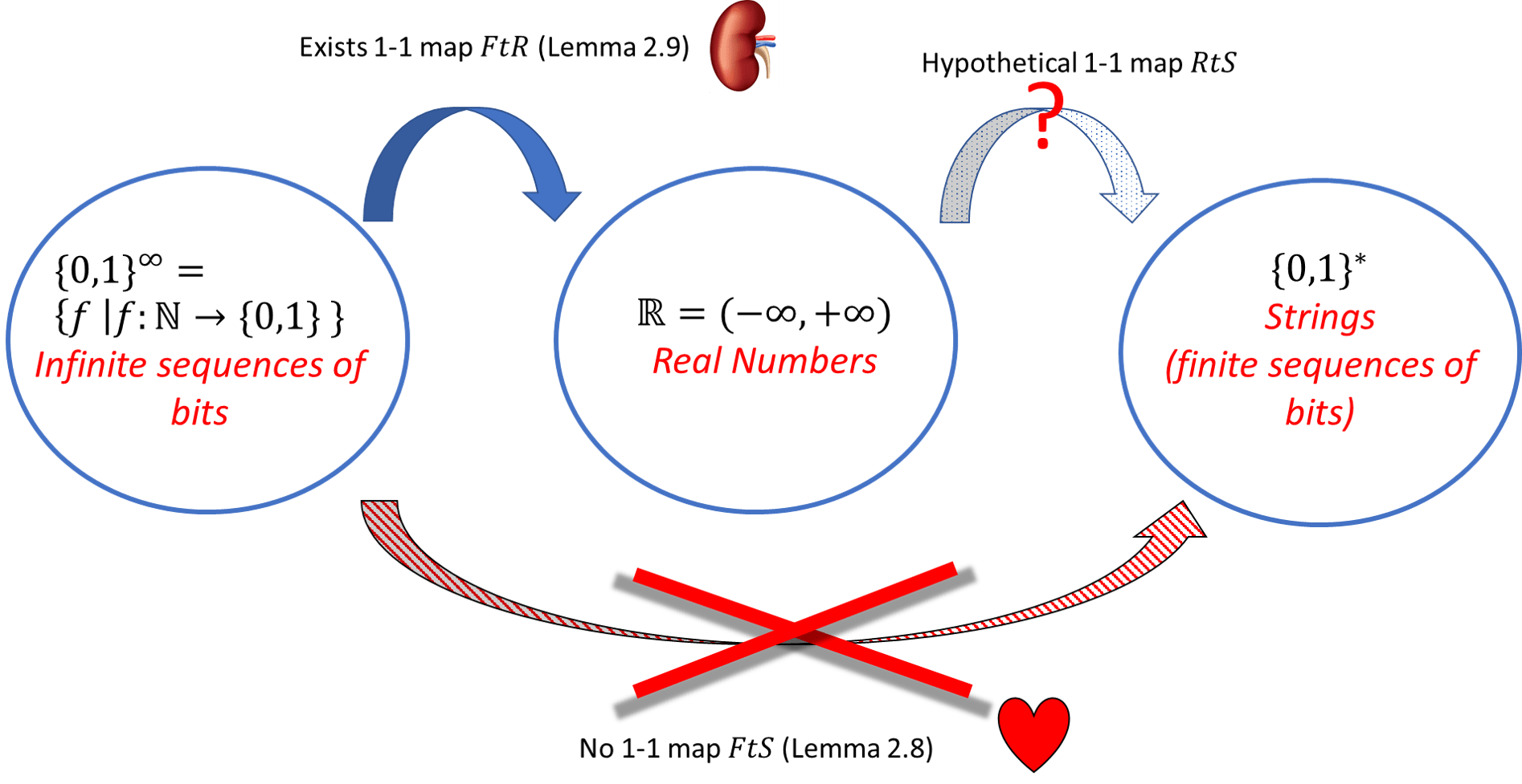
There does not exist a one-to-one map \(FtS:\{0,1\}^\infty \rightarrow \{0,1\}^*\).3
There does exist a one-to-one map \(FtR:\{0,1\}^\infty \rightarrow \R\).4
As we’ve seen above, Lemma 2.8 and Lemma 2.9 together imply Theorem 2.5. To repeat the argument more formally, suppose, for the sake of contradiction, that there did exist a one-to-one function \(RtS:\R \rightarrow \{0,1\}^*\). By Lemma 2.9, there exists a one-to-one function \(FtR:\{0,1\}^\infty \rightarrow \R\). Thus, under this assumption, since the composition of two one-to-one functions is one-to-one (see Exercise 2.12), the function \(FtS:\{0,1\}^\infty \rightarrow \{0,1\}^*\) defined as \(FtS(f)=RtS(FtR(f))\) will be one to one, contradicting Lemma 2.8. See Figure 2.7 for a graphical illustration of this argument.
Now all that is left is to prove these two lemmas. We start by proving Lemma 2.8 which is really the heart of Theorem 2.5.
Warm-up: “Baby Cantor”. The proof of Lemma 2.8 is rather subtle. One way to get intuition for it is to consider the following finite statement “there is no onto function \(f:\{0,\ldots,99\} \rightarrow \{0,1\}^{100}\)”. Of course we know it’s true since the set \(\{0,1\}^{100}\) is bigger than the set \([100]\), but let’s see a direct proof. For every \(f:\{0,\ldots,99\} \rightarrow \{0,1\}^{100}\), we can define the string \(\overline{d} \in \{0,1\}^{100}\) as follows: \(\overline{d} = (1-f(0)_0, 1-f(1)_1 , \ldots, 1-f(99)_{99})\). If \(f\) was onto, then there would exist some \(n\in [100]\) such that \(f(n) =\overline{d}\), but we claim that no such \(n\) exists. Indeed, if there was such \(n\), then the \(n\)-th coordinate of \(\overline{d}\) would equal \(f(n)_n\) but by definition this coordinate equals \(1-f(n)_n\). See also a “proof by code” of this statement.
We will prove that there does not exist an onto function \(StF:\{0,1\}^* \rightarrow \{0,1\}^\infty\). This implies the lemma since for every two sets \(A\) and \(B\), there exists an onto function from \(A\) to \(B\) if and only if there exists a one-to-one function from \(B\) to \(A\) (see Lemma 1.2).
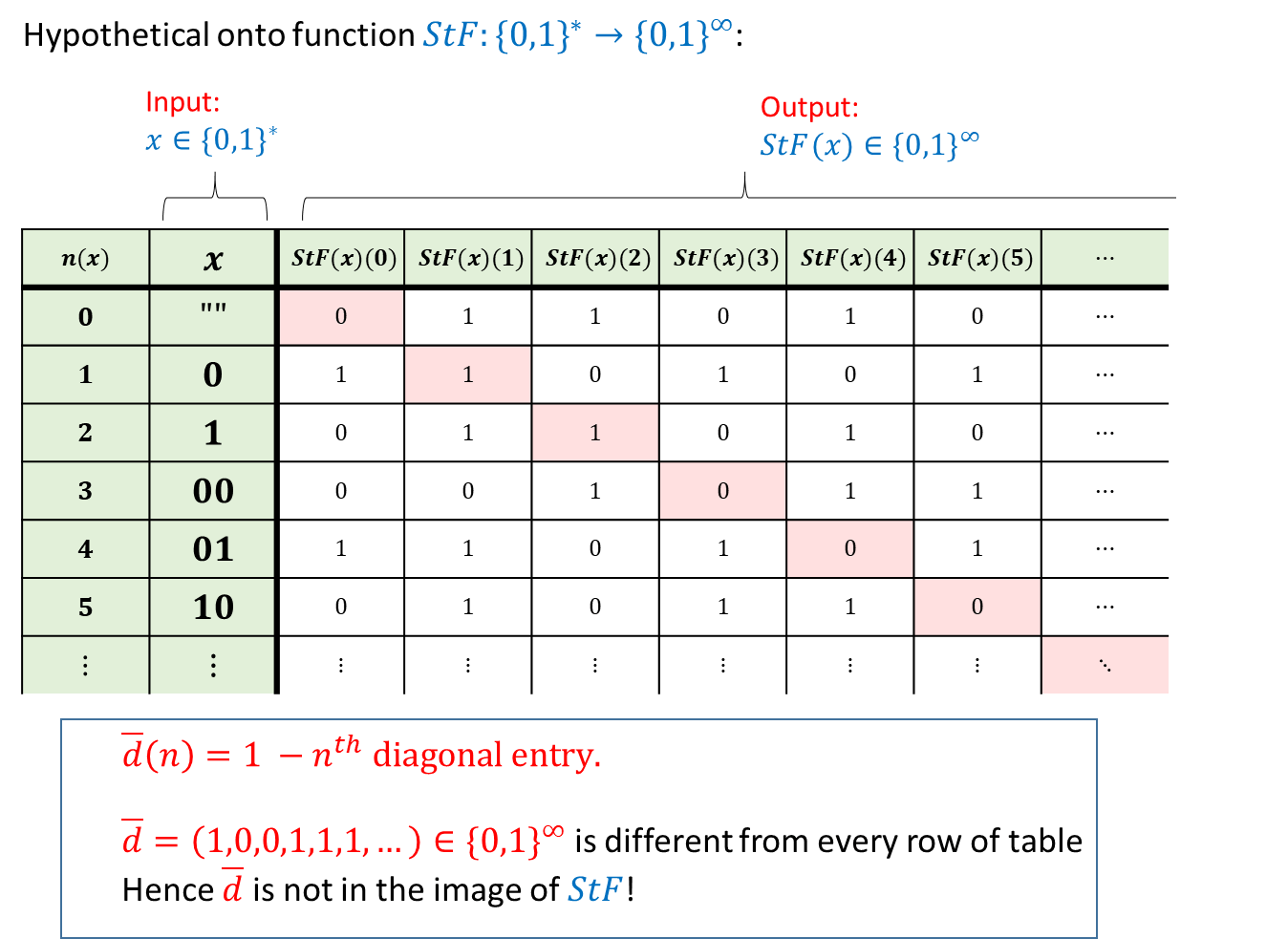
The technique of this proof is known as the “diagonal argument” and is illustrated in Figure 2.8. We assume, towards a contradiction, that there exists such a function \(StF:\{0,1\}^* \rightarrow \{0,1\}^\infty\). We will show that \(StF\) is not onto by demonstrating a function \(\overline{d}\in \{0,1\}^\infty\) such that \(\overline{d} \neq StF(x)\) for every \(x\in \{0,1\}^*\). Consider the lexicographic ordering of binary strings (i.e., \(\ensuremath{\text{\texttt{""}}}\),\(0\),\(1\),\(00\),\(01\),\(\ldots\)). For every \(n\in \N\), we let \(x_n\) be the \(n\)-th string in this order. That is \(x_0 =\ensuremath{\text{\texttt{""}}}\), \(x_1 = 0\), \(x_2= 1\) and so on and so forth. We define the function \(\overline{d} \in \{0,1\}^\infty\) as follows:
The definition of the function \(\overline{d}\) is a bit subtle. One way to think about it is to imagine the function \(StF\) as being specified by an infinitely long table, in which every row corresponds to a string \(x\in \{0,1\}^*\) (with strings sorted in lexicographic order), and contains the sequence \(StF(x)(0), StF(x)(1), StF(x)(2),\ldots\). The diagonal elements in this table are the values
which correspond to the elements \(StF(x_n)(n)\) in the \(n\)-th row and \(n\)-th column of this table for \(n=0,1,2,\ldots\). The function \(\overline{d}\) we defined above maps every \(n\in \N\) to the negation of the \(n\)-th diagonal value.
To complete the proof that \(StF\) is not onto we need to show that \(\overline{d} \neq StF(x)\) for every \(x\in \{0,1\}^*\). Indeed, let \(x\in \{0,1\}^*\) be some string and let \(g = StF(x)\). If \(n\) is the position of \(x\) in the lexicographical order then by construction \(\overline{d}(n) = 1-g(n) \neq g(n)\) which means that \(g \neq \overline{d}\) which is what we wanted to prove.
Lemma 2.8 doesn’t really have much to do with the natural numbers or the strings. An examination of the proof shows that it really shows that for every set \(S\), there is no one-to-one map \(F:\{0,1\}^S \rightarrow S\) where \(\{0,1\}^S\) denotes the set \(\{ f \;|\; f:S \rightarrow \{0,1\} \}\) of all Boolean functions with domain \(S\). Since we can identify a subset \(V \subseteq S\) with its characteristic function \(f=1_V\) (i.e., \(1_V(x)=1\) iff \(x\in V\)), we can think of \(\{0,1\}^S\) also as the set of all subsets of \(S\). This subset is sometimes called the power set of \(S\) and denoted by \(\mathcal{P}(S)\) or \(2^S\).
The proof of Lemma 2.8 can be generalized to show that there is no one-to-one map between a set and its power set. In particular, it means that the set \(\{0,1\}^\R\) is “even bigger” than \(\R\). Cantor used these ideas to construct an infinite hierarchy of shades of infinity. The number of such shades turns out to be much larger than \(|\N|\) or even \(|\R|\). He denoted the cardinality of \(\N\) by \(\aleph_0\) and denoted the next largest infinite number by \(\aleph_1\). (\(\aleph\) is the first letter in the Hebrew alphabet.) Cantor also made the continuum hypothesis that \(|\R|=\aleph_1\). We will come back to the fascinating story of this hypothesis later on in this book. This lecture of Aaronson mentions some of these issues (see also this Berkeley CS 70 lecture).
To complete the proof of Theorem 2.5, we need to show Lemma 2.9. This requires some calculus background but is otherwise straightforward. If you have not had much experience with limits of a real series before, then the formal proof below might be a little hard to follow. This part is not the core of Cantor’s argument, nor are such limits important to the remainder of this book, so you can feel free to take Lemma 2.9 on faith and skip the proof.
We define \(FtR(f)\) to be the number between \(0\) and \(2\) whose decimal expansion is \(f(0).f(1) f(2) \ldots\), or in other words \(FtR(f) = \sum_{i=0}^{\infty} f(i) \cdot 10^{-i}\). If \(f\) and \(g\) are two distinct functions in \(\{0,1\}^\infty\), then there must be some input \(k\) in which they disagree. If we take the minimum such \(k\), then the numbers \(f(0).f(1) f(2) \ldots f(k-1) f(k) \ldots\) and \(g(0) . g(1) g(2) \ldots g(k) \ldots\) agree with each other all the way up to the \(k-1\)-th digit after the decimal point, and disagree on the \(k\)-th digit. But then these numbers must be distinct. Concretely, if \(f(k)=1\) and \(g(k)=0\) then the first number is larger than the second, and otherwise (\(f(k)=0\) and \(g(k)=1\)) the first number is smaller than the second. In the proof we have to be a little careful since these are numbers with infinite expansions. For example, the number one half has two decimal expansions \(0.5\) and \(0.49999\cdots\). However, this issue does not come up here, since we restrict attention only to numbers with decimal expansions that do not involve the digit \(9\).
For every \(f \in \{0,1\}^\infty\), we define \(FtR(f)\) to be the number whose decimal expansion is \(f(0).f(1)f(2)f(3)\ldots\). Formally, It is a known result in calculus (whose proof we will not repeat here) that the series on the right-hand side of Equation 2.2 converges to a definite limit in \(\mathbb{R}\).
We now prove that \(FtR\) is one to one. Let \(f,g\) be two distinct functions in \(\{0,1\}^\infty\). Since \(f\) and \(g\) are distinct, there must be some input on which they differ, and we define \(k\) to be the smallest such input and assume without loss of generality that \(f(k)=0\) and \(g(k)=1\). (Otherwise, if \(f(k)=1\) and \(g(k)=0\), then we can simply switch the roles of \(f\) and \(g\).) The numbers \(FtR(f)\) and \(FtR(g)\) agree with each other up to the \(k-1\)-th digit up after the decimal point. Since this digit equals \(0\) for \(FtR(f)\) and equals \(1\) for \(FtR(g)\), we claim that \(FtR(g)\) is bigger than \(FtR(f)\) by at least \(0.5 \cdot 10^{-k}\). To see this note that the difference \(FtR(g)-FtR(f)\) will be minimized if \(g(\ell)=0\) for every \(\ell>k\) and \(f(\ell)=1\) for every \(\ell>k\), in which case (since \(f\) and \(g\) agree up to the \(k-1\)-th digit)
Since the infinite series \(\sum_{i=0}^{\infty} 10^{-i}\) converges to \(10/9\), it follows that for every such \(f\) and \(g\), \(FtR(g) - FtR(f) \geq 10^{-k} - 10^{-k-1}\cdot (10/9) > 0\). In particular we see that for every distinct \(f,g \in \{0,1\}^\infty\), \(FtR(f) \neq FtR(g)\), implying that the function \(FtR\) is one to one.
In the proof above we used the fact that \(1 + 1/10 + 1/100 + \cdots\) converges to \(10/9\), which plugging into Equation 2.3 yields that the difference between \(FtR(g)\) and \(FtR(h)\) is at least \(10^{-k} - 10^{-k-1}\cdot (10/9) > 0\). While the choice of the decimal representation for \(FtR\) was arbitrary, we could not have used the binary representation in its place. Had we used the binary expansion instead of decimal, the corresponding sequence \(1 + 1/2 + 1/4 + \cdots\) converges to \(2/1=2\), and since \(2^{-k} = 2^{-k-1} \cdot 2\), we could not have deduced that \(FtR\) is one to one. Indeed there do exist pairs of distinct sequences \(f,g\in \{0,1\}^\infty\) such that \(\sum_{i=0}^\infty f(i)2^{-i} = \sum_{i=0}^\infty g(i)2^{-i}\). (For example, the sequence \(1,0,0,0,\ldots\) and the sequence \(0,1,1,1,\ldots\) have this property.)
Corollary: Boolean functions are uncountable
Cantor’s Theorem yields the following corollary that we will use several times in this book: the set of all Boolean functions (mapping \(\{0,1\}^*\) to \(\{0,1\}\)) is not countable:
Let \(\ensuremath{\mathit{ALL}}\) be the set of all functions \(F:\{0,1\}^* \rightarrow \{0,1\}\). Then \(\ensuremath{\mathit{ALL}}\) is uncountable. Equivalently, there does not exist an onto map \(StALL:\{0,1\}^* \rightarrow \ensuremath{\mathit{ALL}}\).
This is a direct consequence of Lemma 2.8, since we can use the binary representation to show a one-to-one map from \(\{0,1\}^\infty\) to \(\ensuremath{\mathit{ALL}}\). Hence the uncountability of \(\{0,1\}^\infty\) implies the uncountability of \(\ensuremath{\mathit{ALL}}\).
Since \(\{0,1\}^\infty\) is uncountable, the result will follow by showing a one-to-one map from \(\{0,1\}^\infty\) to \(\ensuremath{\mathit{ALL}}\). The reason is that the existence of such a map implies that if \(\ensuremath{\mathit{ALL}}\) was countable, and hence there was a one-to-one map from \(\ensuremath{\mathit{ALL}}\) to \(\N\), then there would have been a one-to-one map from \(\{0,1\}^\infty\) to \(\N\), contradicting Lemma 2.8.
We now show this one-to-one map. We simply map a function \(f \in \{0,1\}^\infty\) to the function \(F:\{0,1\}^* \rightarrow \{0,1\}\) as follows. We let \(F(0)=f(0)\), \(F(1)=f(1)\), \(F(10)=f(2)\), \(F(11)=f(3)\) and so on and so forth. That is, for every \(x\in \{0,1\}^*\) that represents a natural number \(n\) in the binary basis, we define \(F(x)=f(n)\). If \(x\) does not represent such a number (e.g., it has a leading zero), then we set \(F(x)=0\).
This map is one-to-one since if \(f \neq g\) are two distinct elements in \(\{0,1\}^\infty\), then there must be some input \(n\in \N\) on which \(f(n) \neq g(n)\). But then if \(x\in \{0,1\}^*\) is the string representing \(n\), we see that \(F(x) \neq G(x)\) where \(F\) is the function in \(\ensuremath{\mathit{ALL}}\) that \(f\) mapped to, and \(G\) is the function that \(g\) is mapped to.
Equivalent conditions for countability
The results above establish many equivalent ways to phrase the fact that a set is countable. Specifically, the following statements are all equivalent:
The set \(S\) is countable
There exists an onto map from \(\N\) to \(S\)
There exists an onto map from \(\{0,1\}^*\) to \(S\).
There exists a one-to-one map from \(S\) to \(\N\)
There exists a one-to-one map from \(S\) to \(\{0,1\}^*\).
There exists an onto map from some countable set \(T\) to \(S\).
There exists a one-to-one map from \(S\) to some countable set \(T\).
Make sure you know how to prove the equivalence of all the results above.
Representing objects beyond numbers
Numbers are of course by no means the only objects that we can represent as binary strings. A representation scheme for representing objects from some set \(\mathcal{O}\) consists of an encoding function that maps an object in \(\mathcal{O}\) to a string, and a decoding function that decodes a string back to an object in \(\mathcal{O}\). Formally, we make the following definition:
Let \(\mathcal{O}\) be any set. A representation scheme for \(\mathcal{O}\) is a pair of functions \(E,D\) where \(E:\mathcal{O} \rightarrow \{0,1\}^*\) is a total one-to-one function, \(D:\{0,1\}^* \rightarrow_p \mathcal{O}\) is a (possibly partial) function, and such that \(D\) and \(E\) satisfy that \(D(E(o))=o\) for every \(o\in \mathcal{O}\). \(E\) is known as the encoding function and \(D\) is known as the decoding function.
Note that the condition \(D(E(o))=o\) for every \(o\in\mathcal{O}\) implies that \(D\) is onto (can you see why?). It turns out that to construct a representation scheme we only need to find an encoding function. That is, every one-to-one encoding function has a corresponding decoding function, as shown in the following lemma:
Suppose that \(E: \mathcal{O} \rightarrow \{0,1\}^*\) is one-to-one. Then there exists a function \(D:\{0,1\}^* \rightarrow \mathcal{O}\) such that \(D(E(o))=o\) for every \(o\in \mathcal{O}\).
Let \(o_0\) be some arbitrary element of \(\mathcal{O}\). For every \(x \in \{0,1\}^*\), there exists either zero or a single \(o\in \mathcal{O}\) such that \(E(o)=x\) (otherwise \(E\) would not be one-to-one). We will define \(D(x)\) to equal \(o_0\) in the first case and this single object \(o\) in the second case. By definition \(D(E(o))=o\) for every \(o\in \mathcal{O}\).
While the decoding function of a representation scheme can in general be a partial function, the proof of Lemma 2.14 implies that every representation scheme has a total decoding function. This observation can sometimes be useful.
Finite representations
If \(\mathcal{O}\) is finite, then we can represent every object in \(\mathcal{O}\) as a string of length at most some number \(n\). What is the value of \(n\)? Let us denote by \(\{0,1\}^{\leq n}\) the set \(\{ x\in \{0,1\}^* : |x| \leq n \}\) of strings of length at most \(n\). The size of \(\{0,1\}^{\leq n}\) is equal to
To obtain a representation of objects in \(\mathcal{O}\) as strings of length at most \(n\) we need to come up with a one-to-one function from \(\mathcal{O}\) to \(\{0,1\}^{\leq n}\). We can do so, if and only if \(|\mathcal{O}| \leq 2^{n+1}-1\) as is implied by the following lemma:
For every two non-empty finite sets \(S,T\), there exists a one-to-one \(E:S \rightarrow T\) if and only if \(|S| \leq |T|\).
Let \(k=|S|\) and \(m=|T|\) and so write the elements of \(S\) and \(T\) as \(S = \{ s_0 , s_1, \ldots, s_{k-1} \}\) and \(T= \{ t_0 , t_1, \ldots, t_{m-1} \}\). We need to show that there is a one-to-one function \(E: S \rightarrow T\) iff \(k \leq m\). For the “if” direction, if \(k \leq m\) we can simply define \(E(s_i)=t_i\) for every \(i\in [k]\). Clearly for \(i \neq j\), \(t_i = E(s_i) \neq E(s_j) = t_j\), and hence this function is one-to-one. In the other direction, suppose that \(k>m\) and \(E: S \rightarrow T\) is some function. Then \(E\) cannot be one-to-one. Indeed, for \(i=0,1,\ldots,m-1\) let us “mark” the element \(t_j=E(s_i)\) in \(T\). If \(t_j\) was marked before, then we have found two objects in \(S\) mapping to the same element \(t_j\). Otherwise, since \(T\) has \(m\) elements, when we get to \(i=m-1\) we mark all the objects in \(T\). Hence, in this case, \(E(s_m)\) must map to an element that was already marked before. (This observation is sometimes known as the “Pigeonhole Principle”: the principle that if you have a pigeon coop with \(m\) holes and \(k>m\) pigeons, then there must be two pigeons in the same hole.)
Prefix-free encoding
When showing a representation scheme for rational numbers, we used the “hack” of encoding the alphabet \(\{ 0,1, \|\}\) to represent tuples of strings as a single string. This is a special case of the general paradigm of prefix-free encoding. The idea is the following: if our representation has the property that no string \(x\) representing an object \(o\) is a prefix (i.e., an initial substring) of a string \(y\) representing a different object \(o'\), then we can represent a list of objects by merely concatenating the representations of all the list members. For example, because in English every sentence ends with a punctuation mark such as a period, exclamation, or question mark, no sentence can be a prefix of another and so we can represent a list of sentences by merely concatenating the sentences one after the other. (English has some complications such as periods used for abbreviations (e.g., “e.g.”) or sentence quotes containing punctuation, but the high level point of a prefix-free representation for sentences still holds.)
It turns out that we can transform every representation to a prefix-free form. This justifies Big Idea 1, and allows us to transform a representation scheme for objects of a type \(T\) to a representation scheme of lists of objects of the type \(T\). By repeating the same technique, we can also represent lists of lists of objects of type \(T\), and so on and so forth. But first let us formally define prefix-freeness:
For two strings \(y,y'\), we say that \(y\) is a prefix of \(y'\) if \(|y| \leq |y'|\) and for every \(i<|y|\), \(y'_i = y_i\).
Let \(\mathcal{O}\) be a non-empty set and \(E:\mathcal{O} \rightarrow \{0,1\}^*\) be a function. We say that \(E\) is prefix-free if \(E(o)\) is non-empty for every \(o\in\mathcal{O}\) and there does not exist a distinct pair of objects \(o, o' \in \mathcal{O}\) such that \(E(o)\) is a prefix of \(E(o')\).
Recall that for every set \(\mathcal{O}\), the set \(\mathcal{O}^*\) consists of all finite length tuples (i.e., lists) of elements in \(\mathcal{O}\). The following theorem shows that if \(E\) is a prefix-free encoding of \(\mathcal{O}\) then by concatenating encodings we can obtain a valid (i.e., one-to-one) representation of \(\mathcal{O}^*\):
Suppose that \(E:\mathcal{O} \rightarrow \{0,1\}^*\) is prefix-free. Then the following map \(\overline{E}:\mathcal{O}^* \rightarrow \{0,1\}^*\) is one to one, for every \((o_0,\ldots,o_{k-1}) \in \mathcal{O}^*\), we define
Theorem 2.18 is an example of a theorem that is a little hard to parse, but in fact is fairly straightforward to prove once you understand what it means. Therefore, I highly recommend that you pause here to make sure you understand the statement of this theorem. You should also try to prove it on your own before proceeding further.
The idea behind the proof is simple. Suppose that for example we want to decode a triple \((o_0,o_1,o_2)\) from its representation \(x= \overline{E}(o_0,o_1,o_2)=E(o_0)E(o_1)E(o_2)\). We will do so by first finding the first prefix \(x_0\) of \(x\) that is a representation of some object. Then we will decode this object, remove \(x_0\) from \(x\) to obtain a new string \(x'\), and continue onwards to find the first prefix \(x_1\) of \(x'\) and so on and so forth (see Exercise 2.9). The prefix-freeness property of \(E\) will ensure that \(x_0\) will in fact be \(E(o_0)\), \(x_1\) will be \(E(o_1)\), etc.
We now show the formal proof. Suppose, towards the sake of contradiction, that there exist two distinct tuples \((o_0,\ldots,o_{k-1})\) and \((o'_0,\ldots,o'_{k'-1})\) such that
We will denote the string \(\overline{E}(o_0,\ldots,o_{k-1})\) by \(\overline{x}\).
Let \(i\) be the first index such that \(o_i \neq o'_i\). (If \(o_i=o'_i\) for all \(i\) then, since we assume the two tuples are distinct, one of them must be larger than the other. In this case we assume without loss of generality that \(k'>k\) and let \(i=k\).) In the case that \(i<k\), we see that the string \(\overline{x}\) can be written in two different ways:
and
where \(x_j = E(o_j) = E(o'_j)\) for all \(j<i\). Let \(\overline{y}\) be the string obtained after removing the prefix \(x_0 \cdots x_{i-1}\) from \(\overline{x}\). We see that \(\overline{y}\) can be written as both \(\overline{y}= E(o_i)s\) for some string \(s\in \{0,1\}^*\) and as \(\overline{y} = E(o'_i)s'\) for some \(s'\in \{0,1\}^*\). But this means that one of \(E(o_i)\) and \(E(o'_i)\) must be a prefix of the other, contradicting the prefix-freeness of \(E\).
In the case that \(i=k\) and \(k'>k\), we get a contradiction in the following way. In this case
which means that \(E(o'_k) \cdots E(o'_{k'-1})\) must correspond to the empty string \(\text{\ensuremath{\text{\texttt{""}}}}\). But in such a case \(E(o'_k)\) must be the empty string, which in particular is the prefix of any other string, contradicting the prefix-freeness of \(E\).
Even if the representation \(E\) of objects in \(\mathcal{O}\) is prefix free, this does not mean that our representation \(\overline{E}\) of lists of such objects will be prefix free as well. In fact, it won’t be: for every three objects \(o,o',o''\) the representation of the list \((o,o')\) will be a prefix of the representation of the list \((o,o',o'')\). However, as we see in Lemma 2.20 below, we can transform every representation into prefix-free form, and so will be able to use that transformation if needed to represent lists of lists, lists of lists of lists, and so on and so forth.
Making representations prefix-free
Some natural representations are prefix-free. For example, every fixed output length representation (i.e., one-to-one function \(E:\mathcal{O} \rightarrow \{0,1\}^n\)) is automatically prefix-free, since a string \(x\) can only be a prefix of an equal-length \(x'\) if \(x\) and \(x'\) are identical. Moreover, the approach we used for representing rational numbers can be used to show the following:
Let \(E:\mathcal{O} \rightarrow \{0,1\}^*\) be a one-to-one function. Then there is a one-to-one prefix-free encoding \(\overline{E}\) such that \(|\overline{E}(o)| \leq 2|E(o)|+2\) for every \(o\in \mathcal{O}\).
For the sake of completeness, we will include the proof below, but it is a good idea for you to pause here and try to prove it on your own, using the same technique we used for representing rational numbers.
The idea behind the proof is to use the map \(0 \mapsto 00\), \(1 \mapsto 11\) to “double” every bit in the string \(x\) and then mark the end of the string by concatenating to it the pair \(01\). If we encode a string \(x\) in this way, it ensures that the encoding of \(x\) is never a prefix of the encoding of a distinct string \(x'\). Formally, we define the function \(\ensuremath{\mathit{PF}}:\{0,1\}^* \rightarrow \{0,1\}^*\) as follows:
To prove the lemma we need to show that (1) \(\overline{E}\) is one-to-one and (2) \(\overline{E}\) is prefix-free. In fact, prefix freeness is a stronger condition than one-to-one (if two strings are equal then in particular one of them is a prefix of the other) and hence it suffices to prove (2), which we now do.
Let \(o \neq o'\) in \(\mathcal{O}\) be two distinct objects. We will prove that \(\overline{E}(o)\) is not a prefix of \(\overline{E}(o')\), or in other words \(\ensuremath{\mathit{PF}}(x)\) is not a prefix of \(\ensuremath{\mathit{PF}}(x')\) where \(x = E(o)\) and \(x'=E(o')\). Since \(E\) is one-to-one, \(x \neq x'\). We will split into three cases, depending on whether \(|x|<|x'|\), \(|x|=|x'|\), or \(|x|>|x'|\). If \(|x|<|x'|\) then the two bits in positions \(2|x|,2|x|+1\) in \(\ensuremath{\mathit{PF}}(x)\) have the value \(01\) but the corresponding bits in \(\ensuremath{\mathit{PF}}(x')\) will equal either \(00\) or \(11\) (depending on the \(|x|\)-th bit of \(x'\)) and hence \(\ensuremath{\mathit{PF}}(x)\) cannot be a prefix of \(\ensuremath{\mathit{PF}}(x')\). If \(|x|=|x'|\) then, since \(x \neq x'\), there must be a coordinate \(i\) in which they differ, meaning that the strings \(\ensuremath{\mathit{PF}}(x)\) and \(\ensuremath{\mathit{PF}}(x')\) differ in the coordinates \(2i,2i+1\), which again means that \(\ensuremath{\mathit{PF}}(x)\) cannot be a prefix of \(\ensuremath{\mathit{PF}}(x')\). If \(|x|>|x'|\) then \(|\ensuremath{\mathit{PF}}(x)|=2|x|+2>|\ensuremath{\mathit{PF}}(x')|=2|x'|+2\) and hence \(\ensuremath{\mathit{PF}}(x)\) is longer than (and cannot be a prefix of) \(\ensuremath{\mathit{PF}}(x')\). In all cases we see that \(\ensuremath{\mathit{PF}}(x)=\overline{E}(o)\) is not a prefix of \(\ensuremath{\mathit{PF}}(x')=\overline{E}(o')\), hence completing the proof.
The proof of Lemma 2.20 is not the only or even the best way to transform an arbitrary representation into prefix-free form. Exercise 2.10 asks you to construct a more efficient prefix-free transformation satisfying \(|\overline{E}(o)| \leq |E(o)| + O(\log |E(o)|)\).
“Proof by Python” (optional)
The proofs of Theorem 2.18 and Lemma 2.20 are constructive in the sense that they give us:
A way to transform the encoding and decoding functions of any representation of an object \(O\) to encoding and decoding functions that are prefix-free, and
A way to extend prefix-free encoding and decoding of single objects to encoding and decoding of lists of objects by concatenation.
Specifically, we could transform any pair of Python functions encode and decode to functions pfencode and pfdecode that correspond to a prefix-free encoding and decoding. Similarly, given pfencode and pfdecode for single objects, we can extend them to encoding of lists. Let us show how this works for the case of the NtS and StN functions we defined above.
We start with the “Python proof” of Lemma 2.20: a way to transform an arbitrary representation into one that is prefix free. The function prefixfree below takes as input a pair of encoding and decoding functions, and returns a triple of functions containing prefix-free encoding and decoding functions, as well as a function that checks whether a string is a valid encoding of an object.
# takes functions encode and decode mapping
# objects to lists of bits and vice versa,
# and returns functions pfencode and pfdecode that
# maps objects to lists of bits and vice versa
# in a prefix-free way.
# Also returns a function pfvalid that says
# whether a list is a valid encoding
def prefixfree(encode, decode):
    def pfencode(o):
        L = encode(o)
        return [L[i//2] for i in range(2*len(L))]+[0,1]
    def pfdecode(L):
        return decode([L[j] for j in range(0,len(L)-2,2)])
    def pfvalid(L):
        return (len(L) % 2 == 0 ) and all(L[2*i]==L[2*i+1] for i in range((len(L)-2)//2)) and L[-2:]==[0,1]

    return pfencode, pfdecode, pfvalid

pfNtS, pfStN , pfvalidN = prefixfree(NtS,StN)

NtS(234)
# 11101010
pfNtS(234)
# 111111001100110001
pfStN(pfNtS(234))
# 234
pfvalidM(pfNtS(234))
# true
Note that the Python function prefixfree above takes two Python functions as input and outputs three Python functions as output. (When it’s not too awkward, we use the term “Python function” or “subroutine” to distinguish between such snippets of Python programs and mathematical functions.) You don’t have to know Python in this course, but you do need to get comfortable with the idea of functions as mathematical objects in their own right, that can be used as inputs and outputs of other functions.
We now show a “Python proof” of Theorem 2.18. Namely, we show a function represlists that takes as input a prefix-free representation scheme (implemented via encoding, decoding, and validity testing functions) and outputs a representation scheme for lists of such objects. If we want to make this representation prefix-free then we could fit it into the function prefixfree above.
def represlists(pfencode,pfdecode,pfvalid):
    """
    Takes functions pfencode, pfdecode and pfvalid,
    and returns functions encodelists, decodelists
    that can encode and decode lists of the objects
    respectively.
    """

    def encodelist(L):
        """Gets list of objects, encodes it as list of bits"""
        return "".join([pfencode(obj) for obj in L])

    def decodelist(S):
        """Gets lists of bits, returns lists of objects"""
        i=0; j=1 ; res = []
        while j<=len(S):
            if pfvalid(S[i:j]):
                res += [pfdecode(S[i:j])]
                i=j
            j+= 1
        return res

    return encodelist,decodelist


LtS , StL = represlists(pfNtS,pfStN,pfvalidN)

LtS([234,12,5])
# 111111001100110001111100000111001101
StL(LtS([234,12,5]))
# [234, 12, 5]
Representing letters and text
We can represent a letter or symbol by a string, and then if this representation is prefix-free, we can represent a sequence of symbols by merely concatenating the representation of each symbol. One such representation is the ASCII that represents \(128\) letters and symbols as strings of \(7\) bits. Since the ASCII representation is fixed-length, it is automatically prefix-free (can you see why?). Unicode is the representation of (at the time of this writing) about 128,000 symbols as numbers (known as code points) between \(0\) and \(1,114,111\). There are several types of prefix-free representations of the code points, a popular one being UTF-8 that encodes every codepoint into a string of length between \(8\) and \(32\).
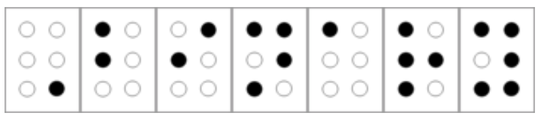
The Braille system is another way to encode letters and other symbols as binary strings. Specifically, in Braille, every letter is encoded as a string in \(\{0,1\}^6\), which is written using indented dots arranged in two columns and three rows, see Figure 2.10. (Some symbols require more than one six-bit string to encode, and so Braille uses a more general prefix-free encoding.)
The Braille system was invented in 1821 by Louis Braille when he was just 12 years old (though he continued working on it and improving it throughout his life). Braille was a French boy who lost his eyesight at the age of 5 as the result of an accident.
We can use programming languages to probe how our computing environment represents various values. This is easiest to do in “unsafe” programming languages such as C that allow direct access to the memory.
Using a simple C program we have produced the following representations of various values. One can see that for integers, multiplying by 2 corresponds to a “left shift” inside each byte. In contrast, for floating-point numbers, multiplying by two corresponds to adding one to the exponent part of the representation. In the architecture we used, a negative number is represented using the two’s complement approach. C represents strings in a prefix-free form by ensuring that a zero byte is at their end.
int      2    : 00000010 00000000 00000000 00000000
int      4    : 00000100 00000000 00000000 00000000
int      513  : 00000001 00000010 00000000 00000000
long     513  : 00000001 00000010 00000000 00000000 00000000 00000000 00000000 00000000
int      -1   : 11111111 11111111 11111111 11111111
int      -2   : 11111110 11111111 11111111 11111111
string   Hello: 01001000 01100101 01101100 01101100 01101111 00000000
string   abcd : 01100001 01100010 01100011 01100100 00000000
float    33.0 : 00000000 00000000 00000100 01000010
float    66.0 : 00000000 00000000 10000100 01000010
float    132.0: 00000000 00000000 00000100 01000011
double   132.0: 00000000 00000000 00000000 00000000 00000000 10000000 01100000 01000000
Representing vectors, matrices, images
Once we can represent numbers and lists of numbers, then we can also represent vectors (which are just lists of numbers). Similarly, we can represent lists of lists, and thus, in particular, can represent matrices. To represent an image, we can represent the color at each pixel by a list of three numbers corresponding to the intensity of Red, Green and Blue. (We can restrict to three primary colors since most humans only have three types of cones in their retinas; we would have needed 16 primary colors to represent colors visible to the Mantis Shrimp.) Thus an image of \(n\) pixels would be represented by a list of \(n\) such length-three lists. A video can be represented as a list of images. Of course these representations are rather wasteful and much more compact representations are typically used for images and videos, though this will not be our concern in this book.
Representing graphs
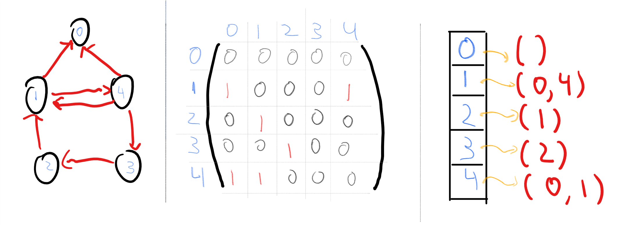
A graph on \(n\) vertices can be represented as an \(n\times n\) adjacency matrix whose \((i,j)^{th}\) entry is equal to \(1\) if the edge \((i,j)\) is present and is equal to \(0\) otherwise. That is, we can represent an \(n\) vertex directed graph \(G=(V,E)\) as a string \(A\in \{0,1\}^{n^2}\) such that \(A_{i,j}=1\) iff the edge \(\overrightarrow{i\;j}\in E\). We can transform an undirected graph to a directed graph by replacing every edge \(\{i,j\}\) with both edges \(\overrightarrow{i\; j}\) and \(\overleftarrow{i\;j}\)
Another representation for graphs is the adjacency list representation. That is, we identify the vertex set \(V\) of a graph with the set \([n]\) where \(n=|V|\), and represent the graph \(G=(V,E)\) as a list of \(n\) lists, where the \(i\)-th list consists of the out-neighbors of vertex \(i\). The difference between these representations can be significant for some applications, though for us would typically be immaterial.
Representing lists and nested lists
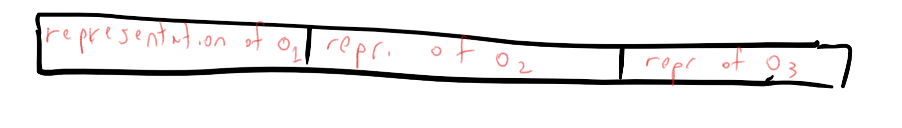
If we have a way of representing objects from a set \(\mathcal{O}\) as binary strings, then we can represent lists of these objects by applying a prefix-free transformation. Moreover, we can use a trick similar to the above to handle nested lists. The idea is that if we have some representation \(E:\mathcal{O} \rightarrow \{0,1\}^*\), then we can represent nested lists of items from \(\mathcal{O}\) using strings over the five element alphabet \(\Sigma = \{\) 0,1,[ , ] , , \(\}\). For example, if \(o_1\) is represented by 0011, \(o_2\) is represented by 10011, and \(o_3\) is represented by 00111, then we can represent the nested list \((o_1,(o_2,o_3))\) as the string "[0011,[10011,00111]]" over the alphabet \(\Sigma\). By encoding every element of \(\Sigma\) itself as a three-bit string, we can transform any representation for objects \(\mathcal{O}\) into a representation that enables representing (potentially nested) lists of these objects.
Notation
We will typically identify an object with its representation as a string. For example, if \(F:\{0,1\}^* \rightarrow \{0,1\}^*\) is some function that maps strings to strings and \(n\) is an integer, we might make statements such as “\(F(n)+1\) is prime” to mean that if we represent \(n\) as a string \(x\), then the integer \(m\) represented by the string \(F(x)\) satisfies that \(m+1\) is prime. (You can see how this convention of identifying objects with their representation can save us a lot of cumbersome formalism.) Similarly, if \(x,y\) are some objects and \(F\) is a function that takes strings as inputs, then by \(F(x,y)\) we will mean the result of applying \(F\) to the representation of the ordered pair \((x,y)\). We use the same notation to invoke functions on \(k\)-tuples of objects for every \(k\).
This convention of identifying an object with its representation as a string is one that we humans follow all the time. For example, when people say a statement such as “\(17\) is a prime number”, what they really mean is that the integer whose decimal representation is the string “17”, is prime.
When we say
\(A\) is an algorithm that computes the multiplication function on natural numbers.
what we really mean is that
\(A\) is an algorithm that computes the function \(F:\{0,1\}^* \rightarrow \{0,1\}^*\) such that for every pair \(a,b \in \N\), if \(x\in \{0,1\}^*\) is a string representing the pair \((a,b)\) then \(F(x)\) will be a string representing their product \(a\cdot b\).
Defining computational tasks as mathematical functions
Abstractly, a computational process is some process that takes an input which is a string of bits and produces an output which is a string of bits. This transformation of input to output can be done using a modern computer, a person following instructions, the evolution of some natural system, or any other means.
In future chapters, we will turn to mathematically defining computational processes, but, as we discussed above, at the moment we focus on computational tasks. That is, we focus on the specification and not the implementation. Again, at an abstract level, a computational task can specify any relation that the output needs to have with the input. However, for most of this book, we will focus on the simplest and most common task of computing a function. Here are some examples:
Given (a representation of) two integers \(x,y\), compute the product \(x\times y\). Using our representation above, this corresponds to computing a function from \(\{0,1\}^*\) to \(\{0,1\}^*\). We have seen that there is more than one way to solve this computational task, and in fact, we still do not know the best algorithm for this problem.
Given (a representation of) an integer \(z>1\), compute its factorization; i.e., the list of primes \(p_1 \leq \cdots \leq p_k\) such that \(z = p_1\cdots p_k\). This again corresponds to computing a function from \(\{0,1\}^*\) to \(\{0,1\}^*\). The gaps in our knowledge of the complexity of this problem are even larger.
Given (a representation of) a graph \(G\) and two vertices \(s\) and \(t\), compute the length of the shortest path in \(G\) between \(s\) and \(t\), or do the same for the longest path (with no repeated vertices) between \(s\) and \(t\). Both these tasks correspond to computing a function from \(\{0,1\}^*\) to \(\{0,1\}^*\), though it turns out that there is a vast difference in their computational difficulty.
Given the code of a Python program, determine whether there is an input that would force it into an infinite loop. This task corresponds to computing a partial function from \(\{0,1\}^*\) to \(\{0,1\}\) since not every string corresponds to a syntactically valid Python program. We will see that we do understand the computational status of this problem, but the answer is quite surprising.
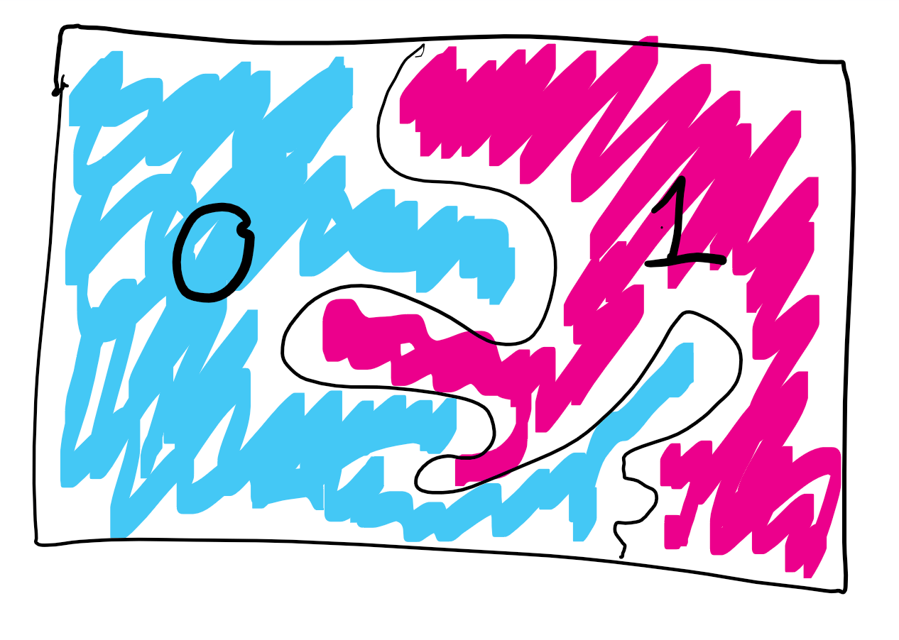
Given (a representation of) an image \(I\), decide if \(I\) is a photo of a cat or a dog. This corresponds to computing some (partial) function from \(\{0,1\}^*\) to \(\{0,1\}\).
An important special case of computational tasks corresponds to computing Boolean functions, whose output is a single bit \(\{0,1\}\). Computing such functions corresponds to answering a YES/NO question, and hence this task is also known as a decision problem. Given any function \(F:\{0,1\}^* \rightarrow \{0,1\}\) and \(x\in \{0,1\}^*\), the task of computing \(F(x)\) corresponds to the task of deciding whether or not \(x\in L\) where \(L = \{ x : F(x)=1 \}\) is known as the language that corresponds to the function \(F\). (The language terminology is due to historical connections between the theory of computation and formal linguistics as developed by Noam Chomsky.) Hence many texts refer to such a computational task as deciding a language.
For every particular function \(F\), there can be several possible algorithms to compute \(F\). We will be interested in questions such as:
For a given function \(F\), can it be the case that there is no algorithm to compute \(F\)?
If there is an algorithm, what is the best one? Could it be that \(F\) is “effectively uncomputable” in the sense that every algorithm for computing \(F\) requires a prohibitively large amount of resources?
If we cannot answer this question, can we show equivalence between different functions \(F\) and \(F'\) in the sense that either they are both easy (i.e., have fast algorithms) or they are both hard?
Can a function being hard to compute ever be a good thing? Can we use it for applications in areas such as cryptography?
In order to do that, we will need to mathematically define the notion of an algorithm, which is what we will do in Chapter 3.
Distinguish functions from programs!
You should always watch out for potential confusions between specifications and implementations or equivalently between mathematical functions and algorithms/programs. It does not help that programming languages (Python included) use the term “functions” to denote (parts of) programs. This confusion also stems from thousands of years of mathematical history, where people typically defined functions by means of a way to compute them.
For example, consider the multiplication function on natural numbers. This is the function \(\ensuremath{\mathit{MULT}}:\N\times \N \rightarrow \N\) that maps a pair \((x,y)\) of natural numbers to the number \(x \cdot y\). As we mentioned, it can be implemented in more than one way:
def mult1(x,y):
    res = 0
    while y>0:
        res += x
        y   -= 1
    return res

def mult2(x,y):
    a = str(x) # represent x as string in decimal notation
    b = str(y) # represent y as string in decimal notation
    res = 0
    for i in range(len(a)):
        for j in range(len(b)):
            res += int(a[len(a)-i])*int(b[len(b)-j])*(10**(i+j))
    return res

print(mult1(12,7))
# 84
print(mult2(12,7))
# 84
Both mult1 and mult2 produce the same output given the same pair of natural number inputs. (Though mult1 will take far longer to do so when the numbers become large.) Hence, even though these are two different programs, they compute the same mathematical function. This distinction between a program or algorithm \(A\), and the function \(F\) that \(A\) computes will be absolutely crucial for us in this course (see also Figure 2.13).
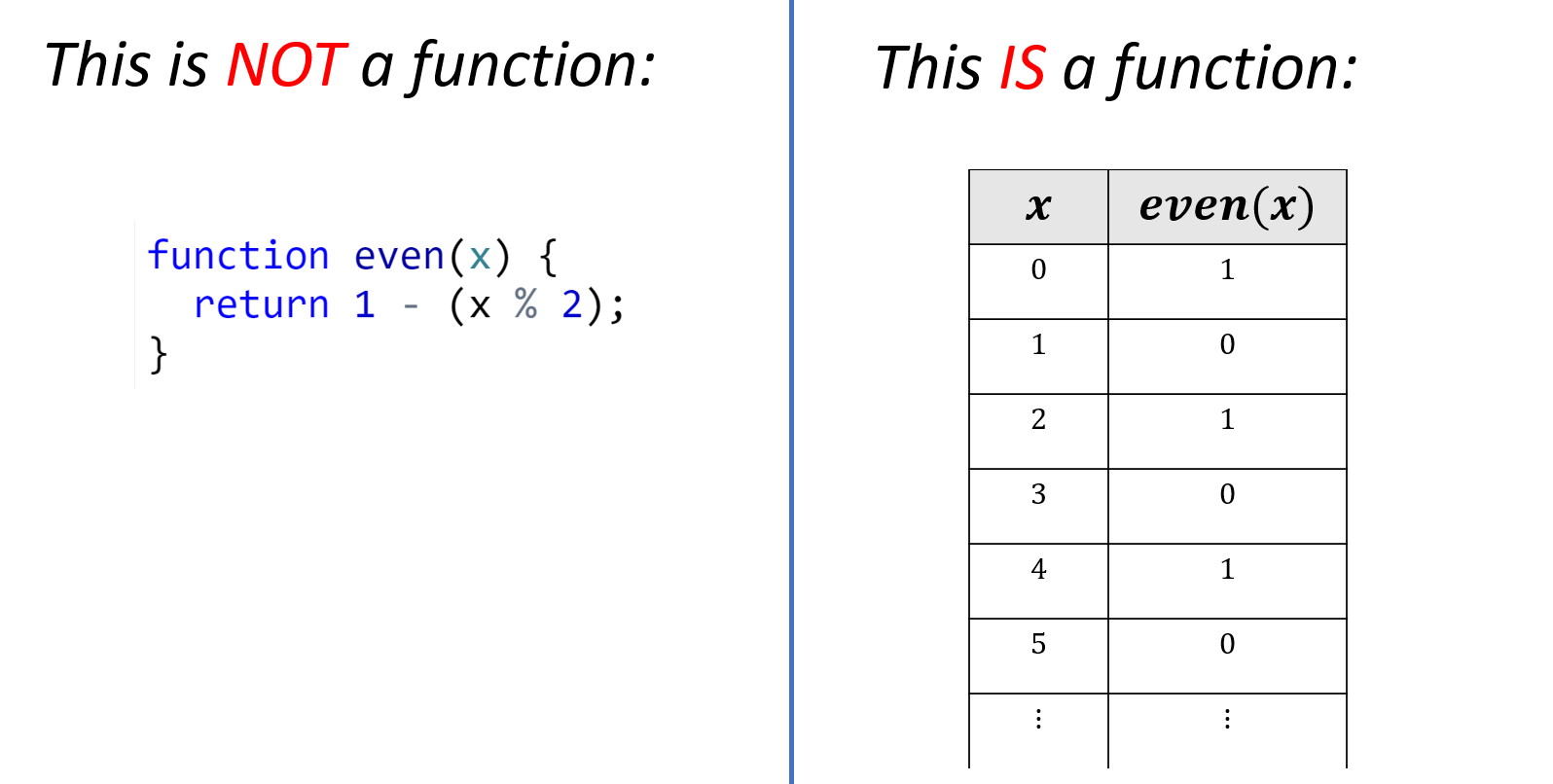
A function is not the same as a program. A program computes a function.
Distinguishing functions from programs (or other ways for computing, including circuits and machines) is a crucial theme for this course. For this reason, this is often a running theme in questions that I (and many other instructors) assign in homework and exams (hint, hint).
Functions capture quite a lot of computational tasks, but one can consider more general settings as well. For starters, we can and will talk about partial functions, that are not defined on all inputs. When computing a partial function, we only need to worry about the inputs on which the function is defined. Another way to say it is that we can design an algorithm for a partial function \(F\) under the assumption that someone “promised” us that all inputs \(x\) would be such that \(F(x)\) is defined (as otherwise, we do not care about the result). Hence such tasks are also known as promise problems.
Another generalization is to consider relations that may have more than one possible admissible output. For example, consider the task of finding any solution for a given set of equations. A relation \(R\) maps a string \(x\in \{0,1\}^*\) into a set of strings \(R(x)\) (for example, \(x\) might describe a set of equations, in which case \(R(x)\) would correspond to the set of all solutions to \(x\)). We can also identify a relation \(R\) with the set of pairs of strings \((x,y)\) where \(y\in R(x)\). A computational process solves a relation if for every \(x\in \{0,1\}^*\), it outputs some string \(y\in R(x)\).
Later in this book, we will consider even more general tasks, including interactive tasks, such as finding a good strategy in a game, tasks defined using probabilistic notions, and others. However, for much of this book, we will focus on the task of computing a function, and often even a Boolean function, that has only a single bit of output. It turns out that a great deal of the theory of computation can be studied in the context of this task, and the insights learned are applicable in the more general settings.
- We can represent objects we want to compute on using binary strings.
- A representation scheme for a set of objects \(\mathcal{O}\) is a one-to-one map from \(\mathcal{O}\) to \(\{0,1\}^*\).
- We can use prefix-free encoding to “boost” a representation for a set \(\mathcal{O}\) into representations of lists of elements in \(\mathcal{O}\).
- A basic computational task is the task of computing a function \(F:\{0,1\}^* \rightarrow \{0,1\}^*\). This task encompasses not just arithmetical computations such as multiplication, factoring, etc. but a great many other tasks arising in areas as diverse as scientific computing, artificial intelligence, image processing, data mining and many many more.
- We will study the question of finding (or at least giving bounds on) what the best algorithm for computing \(F\) for various interesting functions \(F\) is.
Exercises
Which one of these objects can be represented by a binary string?
An integer \(x\)
An undirected graph \(G\).
A directed graph \(H\)
All of the above.
Prove that the function \(NtS:\N \rightarrow \{0,1\}^*\) of the binary representation defined in Equation 2.1 satisfies that for every \(n\in \N\), if \(x = NtS(n)\) then \(|x| =1+\max(0,\floor{\log_2 n})\) and \(x_i = \floor{x/2^{\floor{\log_2 n}-i}} \mod 2\).
Prove that \(NtS\) is a one to one function by coming up with a function \(StN:\{0,1\}^* \rightarrow \N\) such that \(StN(NtS(n))=n\) for every \(n\in \N\).
The ASCII encoding can be used to encode a string of \(n\) English letters as a \(7n\) bit binary string, but in this exercise, we ask about finding a more compact representation for strings of English lowercase letters.
Prove that there exists a representation scheme \((E,D)\) for strings over the 26-letter alphabet \(\{ a, b,c,\ldots,z \}\) as binary strings such that for every \(n>0\) and length-\(n\) string \(x \in \{ a,b,\ldots,z \}^n\), the representation \(E(x)\) is a binary string of length at most \(4.8n+1000\). In other words, prove that for every \(n\), there exists a one-to-one function \(E:\{a,b,\ldots, z\}^n \rightarrow \{0,1\}^{\lfloor 4.8n +1000 \rfloor}\).
Prove that there exists no representation scheme for strings over the alphabet \(\{ a, b,\ldots,z \}\) as binary strings such that for every length-\(n\) string \(x \in \{ a,b,\ldots, z\}^n\), the representation \(E(x)\) is a binary string of length \(\lfloor 4.6n+1000 \rfloor\). In other words, prove that there exists some \(n>0\) such that there is no one-to-one function \(E:\{a,b,\ldots,z \}^n \rightarrow \{0,1\}^{\lfloor 4.6n + 1000 \rfloor}\).
Python’s
bz2.compressfunction is a mapping from strings to strings, which uses the lossless (and hence one to one) bzip2 algorithm for compression. After converting to lowercase, and truncating spaces and numbers, the text of Tolstoy’s “War and Peace” contains \(n=2,517,262\). Yet, if we runbz2.compresson the string of the text of “War and Peace” we get a string of length \(k=6,274,768\) bits, which is only \(2.49n\) (and in particular much smaller than \(4.6n\)). Explain why this does not contradict your answer to the previous question.Interestingly, if we try to apply
bz2.compresson a random string, we get much worse performance. In my experiments, I got a ratio of about \(4.78\) between the number of bits in the output and the number of characters in the input. However, one could imagine that one could do better and that there exists a company called “Pied Piper” with an algorithm that can losslessly compress a string of \(n\) random lowercase letters to fewer than \(4.6n\) bits.5 Show that this is not the case by proving that for every \(n>100\) and one to one function \(Encode:\{a,\ldots,z\}^{n} \rightarrow \{0,1\}^*\), if we let \(Z\) be the random variable \(|Encode(x)|\) (i.e., the length of \(Encode(x)\)) for \(x\) chosen uniformly at random from the set \(\{a,\ldots,z\}^n\), then the expected value of \(Z\) is at least \(4.6n\).
Show that there is a string representation of directed graphs with vertex set \([n]\) and degree at most \(10\) that uses at most \(1000 n\log n\) bits. More formally, show the following: Suppose we define for every \(n\in\mathbb{N}\), the set \(G_n\) as the set containing all directed graphs (with no self loops) over the vertex set \([n]\) where every vertex has degree at most \(10\). Then, prove that for every sufficiently large \(n\), there exists a one-to-one function \(E:G_n \rightarrow \{0,1\}^{\lfloor 1000 n \log n \rfloor}\).
Define \(S_n\) to be the set of one-to-one and onto functions mapping \([n]\) to \([n]\). Prove that there is a one-to-one mapping from \(S_n\) to \(G_{2n}\), where \(G_{2n}\) is the set defined in Exercise 2.4 above.
In this question you will show that one cannot improve the representation of Exercise 2.4 to length \(o(n \log n)\). Specifically, prove for every sufficiently large \(n\in \mathbb{N}\) there is no one-to-one function \(E:G_n \rightarrow \{0,1\}^{\lfloor 0.001 n \log n \rfloor +1000}\).
Recall that the grade-school algorithm for multiplying two numbers requires \(O(n^2)\) operations. Suppose that instead of using decimal representation, we use one of the following representations \(R(x)\) to represent a number \(x\) between \(0\) and \(10^n-1\). For which one of these representations you can still multiply the numbers in \(O(n^2)\) operations?
The standard binary representation: \(B(x)=(x_0,\ldots,x_{k})\) where \(x = \sum_{i=0}^{k} x_i 2^i\) and \(k\) is the largest number s.t. \(x \geq 2^k\).
The reverse binary representation: \(B(x) = (x_{k},\ldots,x_0)\) where \(x_i\) is defined as above for \(i=0,\ldots,k-1\).
Binary coded decimal representation: \(B(x)=(y_0,\ldots,y_{n-1})\) where \(y_i \in \{0,1\}^4\) represents the \(i^{th}\) decimal digit of \(x\) mapping \(0\) to \(0000\), \(1\) to \(0001\), \(2\) to \(0010\), etc. (i.e. \(9\) maps to \(1001\))
All of the above.
Suppose that \(R:\N \rightarrow \{0,1\}^*\) corresponds to representing a number \(x\) as a string of \(x\) \(1\)’s, (e.g., \(R(4)=1111\), \(R(7)=1111111\), etc.). If \(x,y\) are numbers between \(0\) and \(10^n -1\), can we still multiply \(x\) and \(y\) using \(O(n^2)\) operations if we are given them in the representation \(R(\cdot)\)?
Recall that if \(F\) is a one-to-one and onto function mapping elements of a finite set \(U\) into a finite set \(V\) then the sizes of \(U\) and \(V\) are the same. Let \(B:\N\rightarrow\{0,1\}^*\) be the function such that for every \(x\in\N\), \(B(x)\) is the binary representation of \(x\).
Prove that \(x < 2^k\) if and only if \(|B(x)| \leq k\).
Use 1. to compute the size of the set \(\{ y \in \{0,1\}^* : |y| \leq k \}\) where \(|y|\) denotes the length of the string \(y\).
Use 1. and 2. to prove that \(2^k-1 = 1 + 2 + 4+ \cdots + 2^{k-1}\).
Suppose that \(F:\N\rightarrow\{0,1\}^*\) is a one-to-one function that is prefix-free in the sense that there is no \(a\neq b\) s.t. \(F(a)\) is a prefix of \(F(b)\).
Prove that \(F_2:\N\times \N \rightarrow \{0,1\}^*\), defined as \(F_2(a,b) = F(a)F(b)\) (i.e., the concatenation of \(F(a)\) and \(F(b)\)) is a one-to-one function.
Prove that \(F_*:\N^*\rightarrow\{0,1\}^*\) defined as \(F_*(a_1,\ldots,a_k) = F(a_1)\cdots F(a_k)\) is a one-to-one function, where \(\N^*\) denotes the set of all finite-length lists of natural numbers.
Suppose that \(F:O\rightarrow\{0,1\}^*\) is some (not necessarily prefix-free) representation of the objects in the set \(O\), and \(G:\N\rightarrow\{0,1\}^*\) is a prefix-free representation of the natural numbers. Define \(F'(o)=G(|F(o)|)F(o)\) (i.e., the concatenation of the representation of the length \(F(o)\) and \(F(o)\)).
Prove that \(F'\) is a prefix-free representation of \(O\).
Show that we can transform any representation to a prefix-free one by a modification that takes a \(k\) bit string into a string of length at most \(k+O(\log k)\).
Show that we can transform any representation to a prefix-free one by a modification that takes a \(k\) bit string into a string of length at most \(k+ \log k + O(\log\log k)\).6
Suppose that \(S \subseteq \{0,1\}^*\) is some finite prefix-free set, and let \(n\) some number larger than \(\max \{ |x| : x\in X \}\).
For every \(x\in S\), let \(L(x) \subseteq \{0,1\}^n\) denote all the length-\(n\) strings whose first \(k\) bits are \(x_0,\ldots,x_{k-1}\). Prove that (1) \(|L(x)|=2^{n-|x|}\) and (2) For every distinct \(x,x' \in S\), \(L(x)\) is disjoint from \(L(x')\).
Prove that \(\sum_{x\in S}2^{-|x|} \leq 1\). (Hint: first show that \(\sum_{x \in S} |L(x)| \leq 2^n\).)
Prove that there is no prefix-free encoding of strings with less than logarithmic overhead. That is, prove that there is no function \(\ensuremath{\mathit{PF}}:\{0,1\}^* \rightarrow \{0,1\}^*\) s.t. \(|\ensuremath{\mathit{PF}}(x)| \leq |x|+0.9\log |x|\) for every sufficiently large \(x\in \{0,1\}^*\) and such that the set \(\{ \ensuremath{\mathit{PF}}(x) : x\in \{0,1\}^* \}\) is prefix-free. The factor \(0.9\) is arbitrary; all that matters is that it is less than \(1\).
Prove that for every two one-to-one functions \(F:S \rightarrow T\) and \(G:T \rightarrow U\), the function \(H:S \rightarrow U\) defined as \(H(x)=G(F(x))\) is one to one.
We have shown that the natural numbers can be represented as strings. Prove that the other direction holds as well: that there is a one-to-one map \(StN:\{0,1\}^* \rightarrow \N\). (\(StN\) stands for “strings to numbers.”)
Recall that Cantor proved that there is no one-to-one map \(RtN:\R \rightarrow \N\). Show that Cantor’s result implies Theorem 2.5.
Recall that for every set \(S\), the set \(S^*\) is defined as the set of all finite sequences of members of \(S\) (i.e., \(S^* = \{ (x_0,\ldots,x_{n-1}) \;|\; n\in\mathbb{N} \;,\; \forall_{i\in [n]} x_i \in S \}\) ). Prove that there is a one-one-map from \(\mathbb{Z}^*\) to \(\mathbb{N}\) where \(\mathbb{Z}\) is the set of \(\{ \ldots, -3 , -2 , -1,0,+1,+2,+3,\ldots \}\) of all integers.
Bibliographical notes
The study of representing data as strings, including issues such as compression and error corrections falls under the purview of information theory, as covered in the classic textbook of Cover and Thomas (Cover, Thomas, 2006) . Representations are also studied in the field of data structures design, as covered in texts such as (Cormen, Leiserson, Rivest, Stein, 2009) .
The question of whether to represent integers with the most significant digit first or last is known as Big Endian vs. Little Endian representation. This terminology comes from Cohen’s (Cohen, 1981) entertaining and informative paper about the conflict between adherents of both schools which he compared to the warring tribes in Jonathan Swift’s “Gulliver’s Travels”. The two’s complement representation of signed integers was suggested in von Neumann’s classic report (von Neumann, 1945) that detailed the design approaches for a stored-program computer, though similar representations have been used even earlier in abacus and other mechanical computation devices.
The idea that we should separate the definition or specification of a function from its implementation or computation might seem “obvious,” but it took quite a lot of time for mathematicians to arrive at this viewpoint. Historically, a function \(F\) was identified by rules or formulas showing how to derive the output from the input. As we discuss in greater depth in Chapter 9, in the 1800s this somewhat informal notion of a function started “breaking at the seams,” and eventually mathematicians arrived at the more rigorous definition of a function as an arbitrary assignment of input to outputs. While many functions may be described (or computed) by one or more formulas, today we do not consider that to be an essential property of functions, and also allow functions that do not correspond to any “nice” formula.
We have mentioned that all representations of the real numbers are inherently approximate. Thus an important endeavor is to understand what guarantees we can offer on the approximation quality of the output of an algorithm, as a function of the approximation quality of the inputs. This question is known as the question of determining the numerical stability of given equations. The Floating-Point Guide website contains an extensive description of the floating-point representation, as well the many ways in which it could subtly fail, see also the website 0.30000000000000004.com.
Dauben (Dauben, 1990) gives a biography of Cantor with emphasis on the development of his mathematical ideas. (Halmos, 1960) is a classic textbook on set theory, also including Cantor’s theorem. Cantor’s Theorem is also covered in many texts on discrete mathematics, including (Lehman, Leighton, Meyer, 2018) (Lewis, Zax, 2019) .
The adjacency matrix representation of graphs is not merely a convenient way to map a graph into a binary string, but it turns out that many natural notions and operations on matrices are useful for graphs as well. (For example, Google’s PageRank algorithm relies on this viewpoint.) The notes of Spielman’s course are an excellent source for this area, known as spectral graph theory. We will return to this view much later in this book when we talk about random walks.
- ↩
While the Babylonians already invented a positional system much earlier, the decimal positional system we use today was invented by Indian mathematicians around the third century. Arab mathematicians took it up in the 8th century. It first received significant attention in Europe with the publication of the 1202 book “Liber Abaci” by Leonardo of Pisa, also known as Fibonacci, but it did not displace Roman numerals in common usage until the 15th century.
- ↩
\(RtS\) stands for “real numbers to strings”.
- ↩
\(FtS\) stands for “functions to strings”.
- ↩
\(FtR\) stands for “functions to reals.”
- ↩
Actually that particular fictional company uses a metric that focuses more on compression speed then ratio, see here and here.
- ↩
Hint: Think recursively how to represent the length of the string.
Comments
Comments are posted on the GitHub repository using the utteranc.es app. A GitHub login is required to comment. If you don't want to authorize the app to post on your behalf, you can also comment directly on the GitHub issue for this page.
Compiled on 12/06/2023 00:06:46
Copyright 2023, Boaz Barak.

This work is
licensed under a Creative Commons
Attribution-NonCommercial-NoDerivatives 4.0 International License.
Produced using pandoc and panflute with templates derived from gitbook and bookdown.