See any bugs/typos/confusing explanations? Open a GitHub issue. You can also comment below

★ See also the PDF version of this chapter (better formatting/references) ★

Modeling running time

Formally modeling running time, and in particular notions such as $O(n)$ or $O(n^3)$ time algorithms.
The classes $\mathbf{P}$ and $\mathbf{EXP}$ modelling polynomial and exponential time respectively.
The time hierarchy theorem, that in particular says that for every $k \geq 1$ there are functions we can compute in $O(n^{k+1})$ time but can not compute in $O(n^k)$ time.
The class $\mathbf{P_{/poly}}$ of non-uniform computation and the result that $\mathbf{P} \subseteq \mathbf{P_{/poly}}$

“When the measure of the problem-size is reasonable and when the sizes assume values arbitrarily large, an asymptotic estimate of … the order of difficulty of [an] algorithm .. is theoretically important. It cannot be rigged by making the algorithm artificially difficult for smaller sizes”, Jack Edmonds, “Paths, Trees, and Flowers”, 1963

Max Newman: It is all very well to say that a machine could … do this or that, but … what about the time it would take to do it?

Alan Turing: To my mind this time factor is the one question which will involve all the real technical difficulty.

BBC radio panel on “Can automatic Calculating Machines Be Said to Think?”, 1952

In Chapter 12 we saw examples of efficient algorithms, and made some claims about their running time, but did not give a mathematically precise definition for this concept. We do so in this chapter, using the models of Turing machines and RAM machines (or equivalently NAND-TM and NAND-RAM) we have seen before. The running time of an algorithm is not a fixed number since any non-trivial algorithm will take longer to run on longer inputs. Thus, what we want to measure is the dependence between the number of steps the algorithms takes and the length of the input. In particular we care about the distinction between algorithms that take at most polynomial time (i.e., $O(n^c)$ time for some constant $c$) and problems for which every algorithm requires at least exponential time (i.e., $\Omega(2^{n^c})$ for some $c$). As mentioned in Edmond’s quote in Chapter 12, the difference between these two can sometimes be as important as the difference between being computable and uncomputable.

13.1: Overview of the results of this chapter.

In this chapter we formally define what it means for a function to be computable in a certain number of steps. As discussed in Chapter 12, running time is not a number, rather what we care about is the _scaling _behavior of the number of steps as the input size grows. We can use either Turing machines or RAM machines to give such a formal definition - it turns out that this doesn’t make a difference at the resolution we care about. We make several important definitions and prove some important theorems in this chapter. We will define the main time complexity classes we use in this book, and also show the Time Hierarchy Theorem which states that given more resources (more time steps per input size) we can compute more functions.

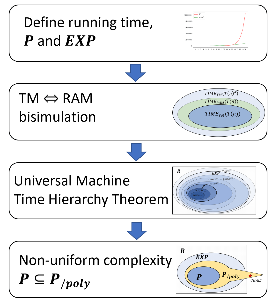
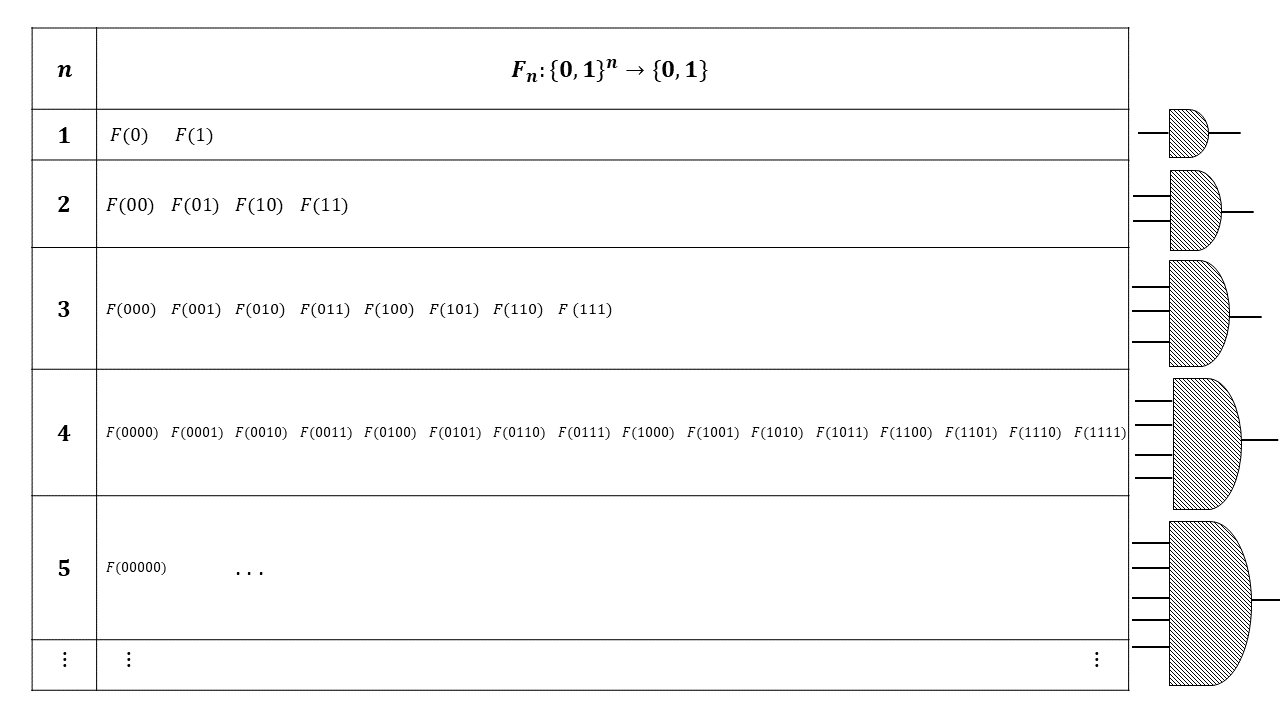
To put this in more “mathy” language, in this chapter we define what it means for a function $F:\{0,1\}^* \rightarrow \{0,1\}^*$ to be computable in time $T(n)$ steps, where $T$ is some function mapping the length $n$ of the input to the number of computation steps allowed. Using this definition we will do the following (see also Figure 13.1):

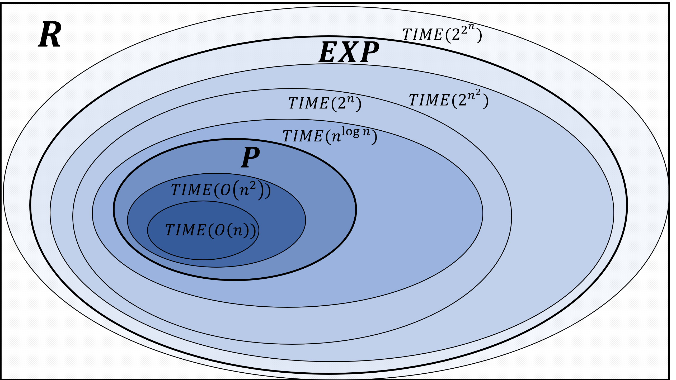
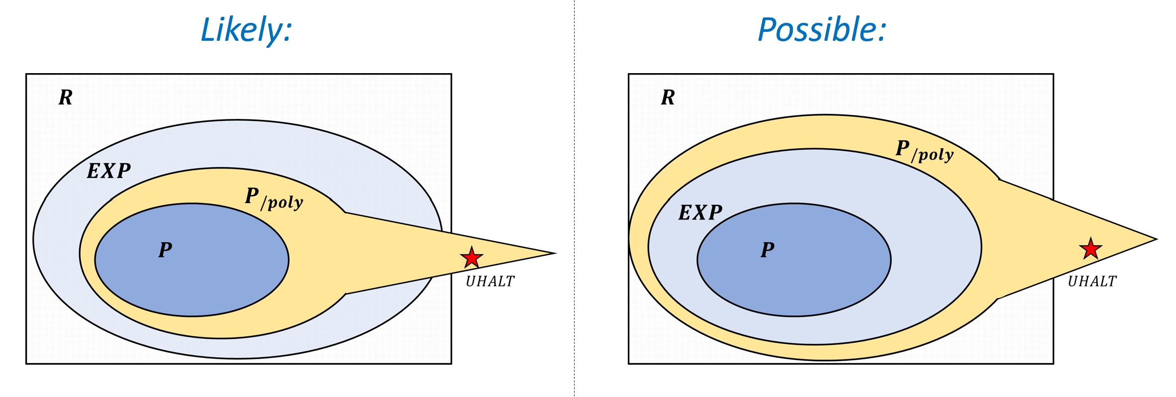
We define the class $\mathbf{P}$ of Boolean functions that can be computed in polynomial time and the class $\mathbf{EXP}$ of functions that can be computed in exponential time. Note that $\mathbf{P} \subseteq \mathbf{EXP}$. If we can compute a function in polynomial time, we can certainly compute it in exponential time.
We show that the times to compute a function using a Turing machine and using a RAM machine (or NAND-RAM program) are polynomially related. In particular this means that the classes $\mathbf{P}$ and $\mathbf{EXP}$ are identical regardless of whether they are defined using Turing machines or RAM machines / NAND-RAM programs.
We give an efficient universal NAND-RAM program and use this to establish the time hierarchy theorem that in particular implies that $\mathbf{P}$ is a strict subset of $\mathbf{EXP}$.
We relate the notions defined here to the non-uniform models of Boolean circuits and NAND-CIRC programs defined in Chapter 3. We define $\mathbf{P_{/poly}}$ to be the class of functions that can be computed by a sequence of polynomial-sized circuits. We prove that $\mathbf{P} \subseteq \mathbf{P_{/poly}}$ and that $\mathbf{P_{/poly}}$ contains uncomputable functions.

Formally defining running time

Our models of computation (Turing machines, NAND-TM and NAND-RAM programs and others) all operate by executing a sequence of instructions on an input one step at a time. We can define the running time of an algorithm $M$ in one of these models by measuring the number of steps $M$ takes on input $x$ as a function of the length $|x|$ of the input. We start by defining running time with respect to Turing machines:

Let $T:\N \rightarrow \N$ be some function mapping natural numbers to natural numbers. We say that a function $F:\{0,1\}^* \rightarrow \{0,1\}^*$ is computable in $T(n)$ Turing-Machine time (TM-time for short) if there exists a Turing machine $M$ such that for every sufficiently large $n$ and every $x\in \{0,1\}^n$, when given input $x$, the machine $M$ halts after executing at most $T(n)$ steps and outputs $F(x)$.

We define $\ensuremath{\mathit{TIME}}_{\mathsf{TM}}(T(n))$ to be the set of Boolean functions (functions mapping $\{0,1\}^*$ to $\{0,1\}$) that are computable in $T(n)$ TM time.

For a function $F:\{0,1\}^* \rightarrow \{0,1\}$ and $T:\N \rightarrow \N$, we can formally define what it means for $F$ to be computable in time at most $T(n)$ where $n$ is the size of the input.

Definition 13.1 is not very complicated but is one of the most important definitions of this book. As usual, $\ensuremath{\mathit{TIME}}_{\mathsf{TM}}(T(n))$ is a class of functions, not of machines. If $M$ is a Turing machine then a statement such as “$M$ is a member of $\ensuremath{\mathit{TIME}}_{\mathsf{TM}}(n^2)$” does not make sense. The concept of TM-time as defined here is sometimes known as “single-tape Turing machine time” in the literature, since some texts consider Turing machines with more than one working tape.

The relaxation of considering only “sufficiently large” $n$’s is not very important but it is convenient since it allows us to avoid dealing explicitly with un-interesting “edge cases”.

While the notion of being computable within a certain running time can be defined for every function, the class $\ensuremath{\mathit{TIME}}_{\mathsf{TM}}(T(n))$ is a class of Boolean functions that have a single bit of output. This choice is not very important, but is made for simplicity and convenience later on. In fact, every non-Boolean function has a computationally equivalent Boolean variant, see Exercise 13.3.

Prove that $\ensuremath{\mathit{TIME}}_{\mathsf{TM}}(10\cdot n^3) \subseteq \ensuremath{\mathit{TIME}}_{\mathsf{TM}}(2^n)$.

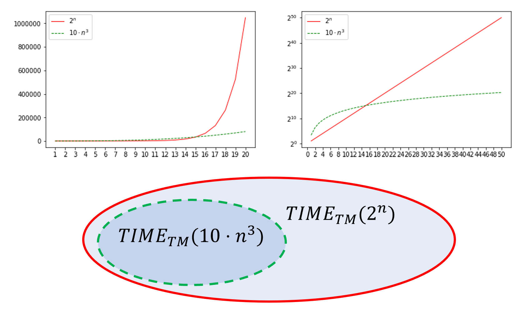
13.2: Comparing $T(n)=10n^3$ with $T'(n) = 2^n$ (on the right figure the Y axis is in log scale). Since for every large enough $n$, $T'(n) \geq T(n)$, $\ensuremath{\mathit{TIME}}_{\mathsf{TM}}(T(n)) \subseteq \ensuremath{\mathit{TIME}}_{\mathsf{TM}}(T'(n))$.

The proof is illustrated in Figure 13.2. Suppose that $F\in \ensuremath{\mathit{TIME}}_{\mathsf{TM}}(10\cdot n^3)$ and hence there exists some number $N_0$ and a machine $M$ such that for every $n> N_0$, and $x\in \{0,1\}^*$, $M(x)$ outputs $F(x)$ within at most $10\cdot n^3$ steps. Since $10\cdot n^3 = o(2^n)$, there is some number $N_1$ such that for every $n>N_1$, $10\cdot n^3 < 2^n$. Hence for every $n > \max\{ N_0, N_1 \}$, $M(x)$ will output $F(x)$ within at most $2^n$ steps, demonstrating that $F \in \ensuremath{\mathit{TIME}}_{\mathsf{TM}}(2^n)$.

Polynomial and Exponential Time

Unlike the notion of computability, the exact running time can be a function of the model we use. However, it turns out that if we only care about “coarse enough” resolution (as will most often be the case) then the choice of the model, whether Turing machines, RAM machines, NAND-TM/NAND-RAM programs, or C/Python programs, does not matter. This is known as the extended Church-Turing Thesis. Specifically we will mostly care about the difference between polynomial and exponential time.

The two main time complexity classes we will be interested in are the following:

Polynomial time: A function $F:\{0,1\}^* \rightarrow \{0,1\}$ is computable in polynomial time if it is in the class $\mathbf{P} = \cup_{c\in \{1,2,3,\ldots \}} \ensuremath{\mathit{TIME}}_{\mathsf{TM}}(n^c)$. That is, $F\in \mathbf{P}$ if there is an algorithm to compute $F$ that runs in time at most polynomial (i.e., at most $n^c$ for some constant $c$) in the length of the input.
Exponential time: A function $F:\{0,1\}^* \rightarrow \{0,1\}$ is computable in exponential time if it is in the class $\mathbf{EXP} = \cup_{c\in \{1,2,3,\ldots \}} \ensuremath{\mathit{TIME}}_{\mathsf{TM}}(2^{n^c})$. That is, $F\in \mathbf{EXP}$ if there is an algorithm to compute $F$ that runs in time at most exponential (i.e., at most $2^{n^c}$ for some constant $c$) in the length of the input.

In other words, these are defined as follows:

Let $F:\{0,1\}^* \rightarrow \{0,1\}$. We say that $F\in \mathbf{P}$ if there is a polynomial $p:\N \rightarrow \R$ and a Turing machine $M$ such that for every $x\in \{0,1\}^*$, when given input $x$, the Turing machine halts within at most $p(|x|)$ steps and outputs $F(x)$.

We say that $F\in \mathbf{EXP}$ if there is a polynomial $p:\N \rightarrow \R$ and a Turing machine $M$ such that for every $x\in \{0,1\}^*$, when given input $x$, $M$ halts within at most $2^{p(|x|)}$ steps and outputs $F(x)$.

Please take the time to make sure you understand these definitions. In particular, sometimes students think of the class $\mathbf{EXP}$ as corresponding to functions that are not in $\mathbf{P}$. However, this is not the case. If $F$ is in $\mathbf{EXP}$ then it can be computed in exponential time. This does not mean that it cannot be computed in polynomial time as well.

Prove that $\mathbf{P}$ as defined in Definition 13.2 is equal to $\cup_{c\in \{1,2,3,\ldots \}} \ensuremath{\mathit{TIME}}_{\mathsf{TM}}(n^c)$

To show these two sets are equal we need to show that $\mathbf{P} \subseteq \cup_{c\in \{1,2,3,\ldots \}} \ensuremath{\mathit{TIME}}_{\mathsf{TM}}(n^c)$ and $\cup_{c\in \{1,2,3,\ldots \}} \ensuremath{\mathit{TIME}}_{\mathsf{TM}}(n^c) \subseteq \mathbf{P}$. We start with the former inclusion. Suppose that $F \in \mathbf{P}$. Then there is some polynomial $p:\N \rightarrow \R$ and a Turing machine $M$ such that $M$ computes $F$ and $M$ halts on every input $x$ within at most $p(|x|)$ steps. We can write the polynomial $p:\N \rightarrow \R$ in the form $p(n) = \sum_{i=0}^d a_i n^i$ where $a_0,\ldots,a_d \in \R$, and we assume that $a_d$ is non-zero (or otherwise we just let $d$ correspond to the largest number such that $a_d$ is non-zero). The degree of $p$ is the number $d$. Since $n^d = o(n^{d+1})$, no matter what the coefficient $a_d$ is, for large enough $n$, $p(n) < n^{d+1}$ which means that the Turing machine $M$ will halt on inputs of length $n$ within fewer than $n^{d+1}$ steps, and hence $F \in \ensuremath{\mathit{TIME}}_{\mathsf{TM}}(n^{d+1}) \subseteq \cup_{c\in \{1,2,3,\ldots \}} \ensuremath{\mathit{TIME}}_{\mathsf{TM}}(n^c)$.

For the second inclusion, suppose that $F \in \cup_{c\in \{1,2,3,\ldots \}} \ensuremath{\mathit{TIME}}_{\mathsf{TM}}(n^c)$. Then there is some positive $c \in \N$ such that $F \in \ensuremath{\mathit{TIME}}_{\mathsf{TM}}(n^c)$ which means that there is a Turing machine $M$ and some number $N_0$ such that $M$ computes $F$ and for every $n>N_0$, $M$ halts on length $n$ inputs within at most $n^c$ steps. Let $T_0$ be the maximum number of steps that $M$ takes on inputs of length at most $N_0$. Then if we define the polynomial $p(n) = n^c + T_0$ then we see that $M$ halts on every input $x$ within at most $p(|x|)$ steps and hence the existence of $M$ demonstrates that $F\in \mathbf{P}$.

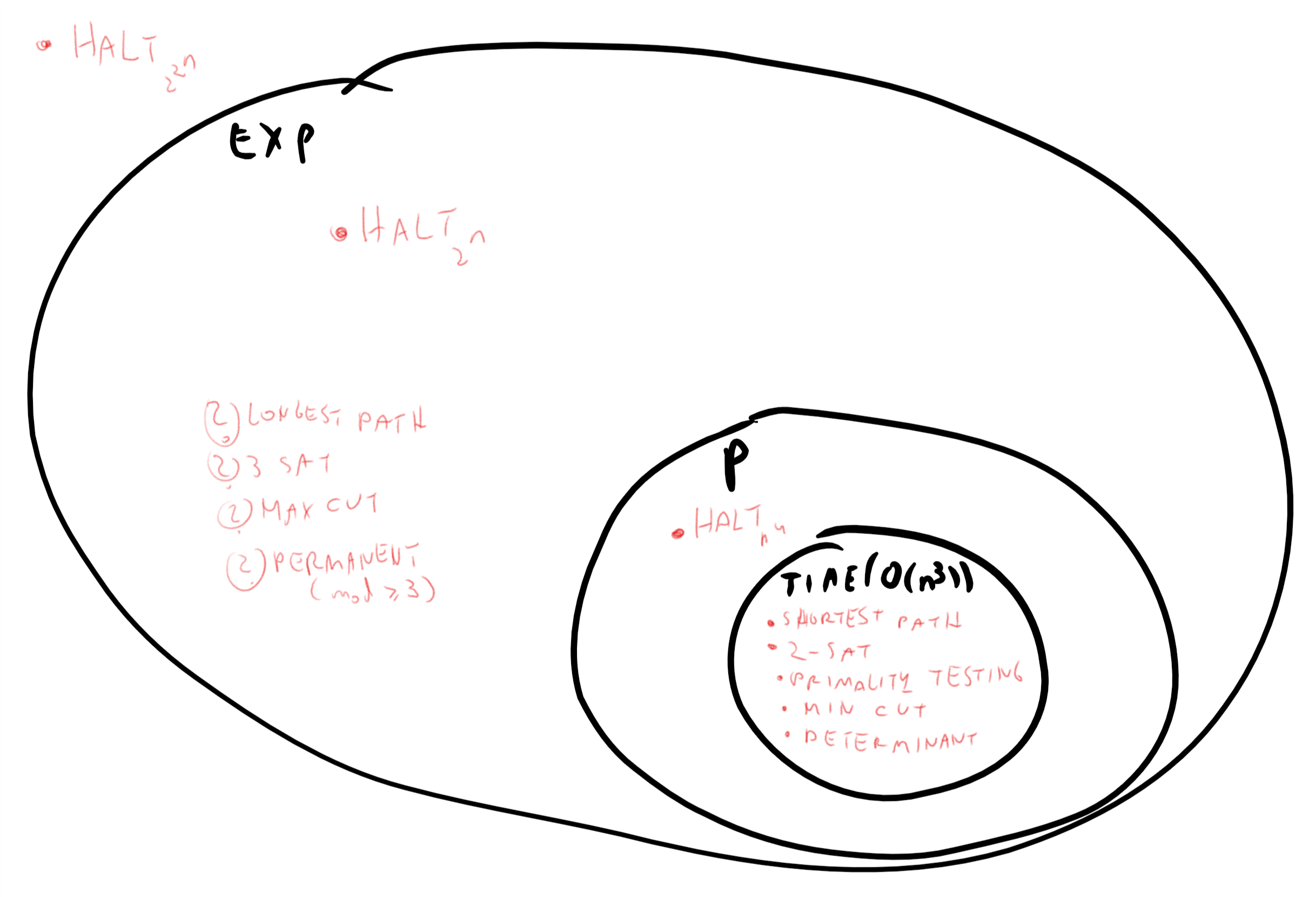
Since exponential time is much larger than polynomial time, $\mathbf{P}\subseteq \mathbf{EXP}$. All of the problems we listed in Chapter 12 are in $\mathbf{EXP}$, but as we’ve seen, for some of them there are much better algorithms that demonstrate that they are in fact in the smaller class $\mathbf{P}$.

$\mathbf{P}$	$\mathbf{EXP}$ (but not known to be in $\mathbf{P}$)
Shortest path	Longest Path
Min cut	Max cut
2SAT	3SAT
Linear eqs	Quad. eqs
Zerosum	Nash
Determinant	Permanent
Primality	Factoring

Table : A table of the examples from Chapter 12. All these problems are in $\mathbf{EXP}$ but only the ones on the left column are currently known to be in $\mathbf{P}$ as well (i.e., they have a polynomial-time algorithm). See also Figure 13.3.

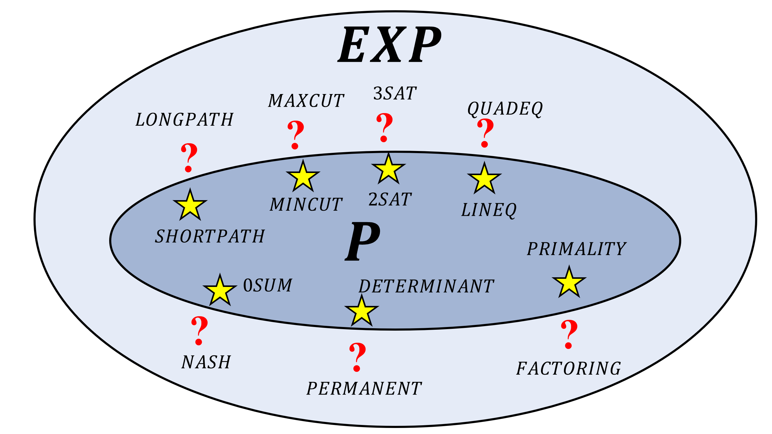
13.3: Some examples of problems that are known to be in $\mathbf{P}$ and problems that are known to be in $\mathbf{EXP}$ but not known whether or not they are in $\mathbf{P}$. Since both $\mathbf{P}$ and $\mathbf{EXP}$ are classes of Boolean functions, in this figure we always refer to the *Boolean* (i.e., Yes/No) variant of the problems.

Many of the problems defined in Chapter 12 correspond to non-Boolean functions (functions with more than one bit of output) while $\mathbf{P}$ and $\mathbf{EXP}$ are sets of Boolean functions. However, for every non-Boolean function $F$ we can always define a computationally-equivalent Boolean function $G$ by letting $G(x,i)$ be the $i$-th bit of $F(x)$ (see Exercise 13.3). Hence the table above, as well as Figure 13.3, refer to the computationally-equivalent Boolean variants of these problems.

Modeling running time using RAM Machines / NAND-RAM

Turing machines are a clean theoretical model of computation, but do not closely correspond to real-world computing architectures. The discrepancy between Turing machines and actual computers does not matter much when we consider the question of which functions are computable, but can make a difference in the context of efficiency. Even a basic staple of undergraduate algorithms such as “merge sort” cannot be implemented on a Turing machine in $O(n\log n)$ time (see Section 13.8). RAM machines (or equivalently, NAND-RAM programs) match more closely actual computing architecture and what we mean when we say $O(n)$ or $O(n \log n)$ algorithms in algorithms courses or whiteboard coding interviews. We can define running time with respect to NAND-RAM programs just as we did for Turing machines.

Let $T:\N \rightarrow \N$ be some function mapping natural numbers to natural numbers. We say that a function $F:\{0,1\}^* \rightarrow \{0,1\}^*$ is computable in $T(n)$ RAM time (RAM-time for short) if there exists a NAND-RAM program $P$ such that for every sufficiently large $n$ and every $x\in \{0,1\}^n$, when given input $x$, the program $P$ halts after executing at most $T(n)$ lines and outputs $F(x)$.

We define $\ensuremath{\mathit{TIME}}_{\mathsf{RAM}}(T(n))$ to be the set of Boolean functions (functions mapping $\{0,1\}^*$ to $\{0,1\}$) that are computable in $T(n)$ RAM time.

Because NAND-RAM programs correspond more closely to our natural notions of running time, we will use NAND-RAM as our “default” model of running time, and hence use $\ensuremath{\mathit{TIME}}(T(n))$ (without any subscript) to denote $\ensuremath{\mathit{TIME}}_{\mathsf{RAM}}(T(n))$. However, it turns out that as long as we only care about the difference between exponential and polynomial time, this does not make much difference. The reason is that Turing machines can simulate NAND-RAM programs with at most a polynomial overhead (see also Figure 13.4):

Let $T:\N \rightarrow \N$ be a function such that $T(n) \geq n$ for every $n$ and the map $n \mapsto T(n)$ can be computed by a Turing machine in time $O(T(n))$. Then

\[ \ensuremath{\mathit{TIME}}_{\mathsf{TM}}(T(n)) \subseteq \ensuremath{\mathit{TIME}}_{\mathsf{RAM}}(10\cdot T(n)) \subseteq \ensuremath{\mathit{TIME}}_{\mathsf{TM}}(T(n)^4) \;. \;\;(13.1) \]

The technical details of Theorem 13.5, such as the condition that $n \mapsto T(n)$ is computable in $O(T(n))$ time or the constants $10$ and $4$ in Equation 13.1 (which are not tight and can be improved), are not very important. In particular, all non-pathological time bound functions we encounter in practice such as $T(n)=n$, $T(n)=n\log n$, $T(n)=2^n$ etc. will satisfy the conditions of Theorem 13.5, see also Remark 13.6.

The main message of the theorem is Turing machines and RAM machines are “roughly equivalent” in the sense that one can simulate the other with polynomial overhead. Similarly, while the proof involves some technical details, it’s not very deep or hard, and merely follows the simulation of RAM machines with Turing machines we saw in Theorem 8.1 with more careful “book keeping”.

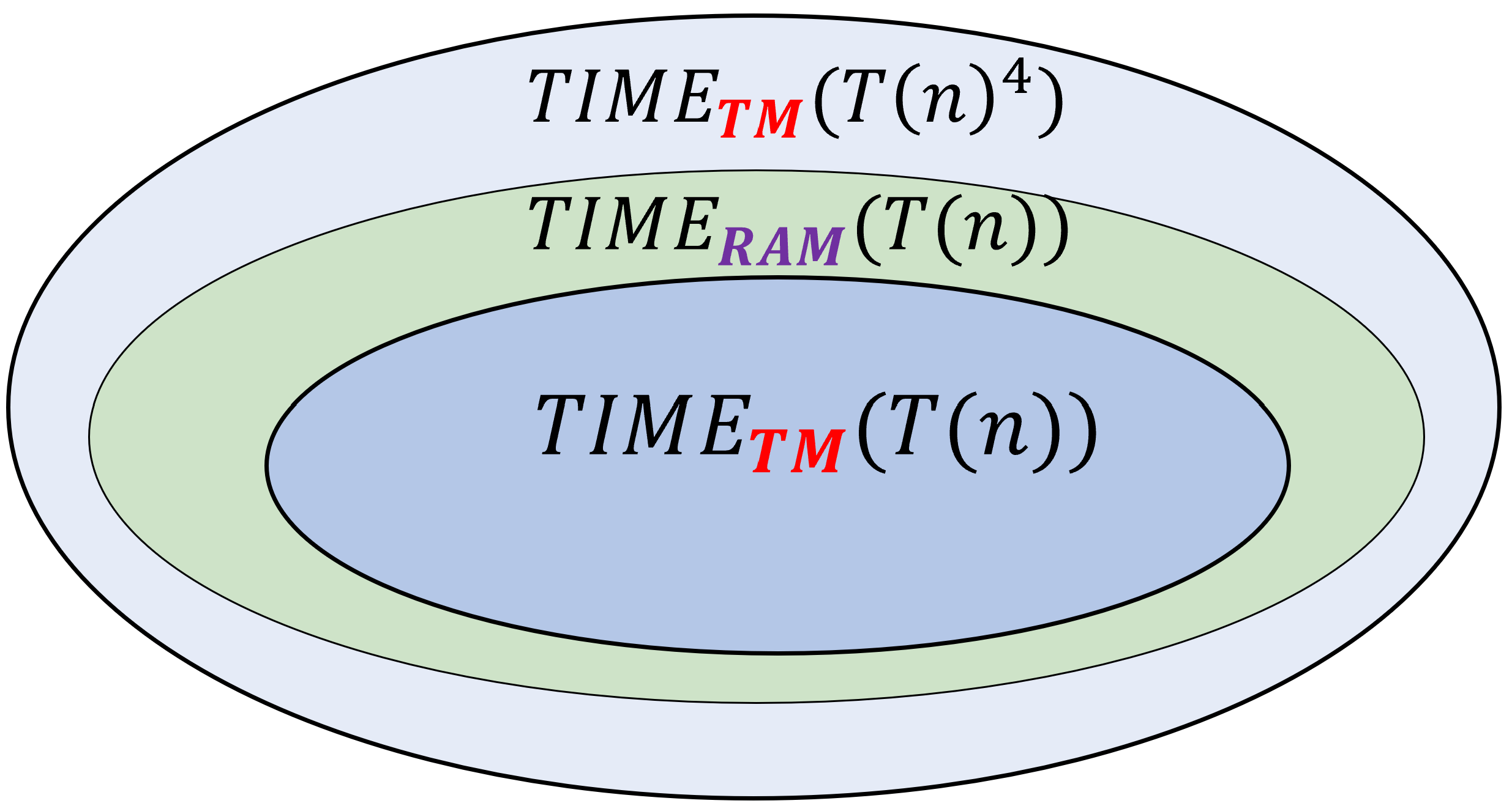
13.4: The proof of Theorem 13.5 shows that we can simulate $T$ steps of a Turing machine with $T$ steps of a NAND-RAM program, and can simulate $T$ steps of a NAND-RAM program with $o(T^4)$ steps of a Turing machine. Hence $\ensuremath{\mathit{TIME}}_{\mathsf{TM}}(T(n)) \subseteq \ensuremath{\mathit{TIME}}_{\mathsf{RAM}}(10\cdot T(n)) \subseteq \ensuremath{\mathit{TIME}}_{\mathsf{TM}}(T(n)^4)$.

For example, by instantiating Theorem 13.5 with $T(n)=n^a$ and using the fact that $10n^a = o(n^{a+1})$, we see that $\ensuremath{\mathit{TIME}}_{\mathsf{TM}}(n^a) \subseteq \ensuremath{\mathit{TIME}}_{\mathsf{RAM}}(n^{a+1}) \subseteq \ensuremath{\mathit{TIME}}_{\mathsf{TM}}(n^{4a+4})$ which means that (by Solved Exercise 13.2)

\[ \mathbf{P} = \cup_{a = 1,2,\ldots} \ensuremath{\mathit{TIME}}_{\mathsf{TM}}(n^a) = \cup_{a = 1,2,\ldots} \ensuremath{\mathit{TIME}}_{\mathsf{RAM}}(n^a) \;. \]

That is, we could have equally well defined $\mathbf{P}$ as the class of functions computable by NAND-RAM programs (instead of Turing machines) that run in time polynomial in the length of the input. Similarly, by instantiating Theorem 13.5 with $T(n)=2^{n^a}$ we see that the class $\mathbf{EXP}$ can also be defined as the set of functions computable by NAND-RAM programs in time at most $2^{p(n)}$ where $p$ is some polynomial. Similar equivalence results are known for many models including cellular automata, C/Python/Javascript programs, parallel computers, and a great many other models, which justifies the choice of $\mathbf{P}$ as capturing a technology-independent notion of tractability. (See Section 13.3 for more discussion of this issue.) This equivalence between Turing machines and NAND-RAM (as well as other models) allows us to pick our favorite model depending on the task at hand (i.e., “have our cake and eat it too”) even when we study questions of efficiency, as long as we only care about the gap between polynomial and exponential time. When we want to design an algorithm, we can use the extra power and convenience afforded by NAND-RAM. When we want to analyze a program or prove a negative result, we can restrict our attention to Turing machines.

All “reasonable” computational models are equivalent if we only care about the distinction between polynomial and exponential.

The adjective “reasonable” above refers to all scalable computational models that have been implemented, with the possible exception of quantum computers, see Section 13.3 and Chapter 23.

The direction $\ensuremath{\mathit{TIME}}_{\mathsf{TM}}(T(n)) \subseteq \ensuremath{\mathit{TIME}}_{\mathsf{RAM}}(10 \cdot T(n))$ is not hard to show, since a NAND-RAM program $P$ can simulate a Turing machine $M$ with constant overhead by storing the transition table of $M$ in an array (as is done in the proof of Theorem 9.1). Simulating every step of the Turing machine can be done in a constant number $c$ of steps of RAM, and it can be shown this constant $c$ is smaller than $10$. Thus the heart of the theorem is to prove that $\ensuremath{\mathit{TIME}}_{\mathsf{RAM}}(T(n)) \subseteq \ensuremath{\mathit{TIME}}_{\mathsf{TM}}(T(n)^4)$. This proof closely follows the proof of Theorem 8.1, where we have shown that every function $F$ that is computable by a NAND-RAM program $P$ is computable by a Turing machine (or equivalently a NAND-TM program) $M$. To prove Theorem 13.5, we follow the exact same proof but just check that the overhead of the simulation of $P$ by $M$ is polynomial. The proof has many details, but is not deep. It is therefore much more important that you understand the statement of this theorem than its proof.

We only focus on the non-trivial direction $\ensuremath{\mathit{TIME}}_{\mathsf{RAM}}(T(n)) \subseteq \ensuremath{\mathit{TIME}}_{\mathsf{TM}}(T(n)^4)$. Let $F\in \ensuremath{\mathit{TIME}}_{\mathsf{RAM}}(T(n))$. $F$ can be computed in time $T(n)$ by some NAND-RAM program $P$ and we need to show that it can also be computed in time $T(n)^4$ by a Turing machine $M$. This will follow from showing that $F$ can be computed in time $T(n)^4$ by a NAND-TM program, since for every NAND-TM program $Q$ there is a Turing machine $M$ simulating it such that each iteration of $Q$ corresponds to a single step of $M$.

As mentioned above, we follow the proof of Theorem 8.1 (simulation of NAND-RAM programs using NAND-TM programs) and use the exact same simulation, but with a more careful accounting of the number of steps that the simulation costs. Recall, that the simulation of NAND-RAM works by “peeling off” features of NAND-RAM one by one, until we are left with NAND-TM.

We will not provide the full details but will present the main ideas used in showing that every feature of NAND-RAM can be simulated by NAND-TM with at most a polynomial overhead:

Recall that every NAND-RAM variable or array element can contain an integer between $0$ and $T$ where $T$ is the number of lines that have been executed so far. Therefore if $P$ is a NAND-RAM program that computes $F$ in $T(n)$ time, then on inputs of length $n$, all integers used by $P$ are of magnitude at most $T(n)$. This means that the largest value i can ever reach is at most $T(n)$ and so each one of $P$’s variables can be thought of as an array of at most $T(n)$ indices, each of which holds a natural number of magnitude at most $T(n)$. We let $\ell = \ceil{\log T(n)}$ be the number of bits needed to encode such numbers. (We can start off the simulation by computing $T(n)$ and $\ell$.)
We can encode a NAND-RAM array of length $\leq T(n)$ containing numbers in $\{0,\ldots, T(n)-1 \}$ as an Boolean (i.e., NAND-TM) array of $T(n)\ell =O(T(n)\log T(n))$ bits, which we can also think of as a two dimensional array as we did in the proof of Theorem 8.1. We encode a NAND-RAM scalar containing a number in $\{0,\ldots, T(n)-1 \}$ simply by a shorter NAND-TM array of $\ell$ bits.
We can simulate the two dimensional arrays using one-dimensional arrays of length $T(n)\ell = O(T(n) \log T(n))$. All the arithmetic operations on integers use the grade-school algorithms, that take time that is polynomial in the number $\ell$ of bits of the integers, which is $poly(\log T(n))$ in our case. Hence we can simulate $T(n)$ steps of NAND-RAM with $O(T(n)poly(\log T(n))$ steps of a model that uses random access memory but only Boolean-valued one-dimensional arrays.
The most expensive step is to translate from random access memory to the sequential memory model of NAND-TM/Turing machines. As we did in the proof of Theorem 8.1 (see Section 8.2), we can simulate accessing an array Foo at some location encoded in an array Bar by:
1. Copying Bar to some temporary array Temp
2. Having an array Index which is initially all zeros except $1$ at the first location.
3. Repeating the following until Temp encodes the number $0$: (Number of repetitions is at most $T(n)$.)
  - Decrease the number encoded temp by $1$. (Takes number of steps polynomial in $\ell = \ceil{\log T(n)}$.)
  - Decrease i until it is equal to $0$. (Takes $O(T(n))$ steps.)
  - Scan Index until we reach the point in which it equals $1$ and then change this $1$ to $0$ and go one step further and write $1$ in this location. (Takes $O(T(n))$ steps.)
4. When we are done we know that if we scan Index until we reach the point in which Index[i]$=1$ then i contains the value that was encoded by Bar (Takes $O(T(n))$ steps.)

The total cost for each such operation is $O(T(n)^2 + T(n)poly(\log T(n))) = O(T(n)^2)$ steps.

In sum, we simulate a single step of NAND-RAM using $O(T(n)^2 poly(\log T(n)))$ steps of NAND-TM, and hence the total simulation time is $O(T(n)^3 poly(\log T(n)))$ which is smaller than $T(n)^4$ for sufficiently large $n$.

When considering general time bounds we need to make sure to rule out some “pathological” cases such as functions $T$ that don’t give enough time for the algorithm to read the input, or functions where the time bound itself is uncomputable. We say that a function $T:\N \rightarrow \N$ is a nice time bound function (or nice function for short) if for every $n\in \N$, $T(n) \geq n$ (i.e., $T$ allows enough time to read the input), for every $n' \geq n$, $T(n') \geq T(n)$ (i.e., $T$ allows more time on longer inputs), and the map $F(x) = 1^{T(|x|)}$ (i.e., mapping a string of length $n$ to a sequence of $T(n)$ ones) can be computed by a NAND-RAM program in $O(T(n))$ time.

All the “normal” time complexity bounds we encounter in applications such as $T(n)= 100 n$, $T(n) = n^2 \log n$,$T(n) = 2^{\sqrt{n}}$, etc. are “nice”. Hence from now on we will only care about the class $\ensuremath{\mathit{TIME}}(T(n))$ when $T$ is a “nice” function. The computability condition is in particular typically easily satisfied. For example, for arithmetic functions such as $T(n) = n^3$, we can typically compute the binary representation of $T(n)$ in time polynomial in the number of bits of $T(n)$ and hence poly-logarithmic in $T(n)$. Hence the time to write the string $1^{T(n)}$ in such cases will be $T(n) + poly(\log T(n)) = O(T(n))$.

Extended Church-Turing Thesis (discussion)

Theorem 13.5 shows that the computational models of Turing machines and RAM machines / NAND-RAM programs are equivalent up to polynomial factors in the running time. Other examples of polynomially equivalent models include:

All standard programming languages, including C/Python/JavaScript/Lisp/etc.
The $\lambda$ calculus (see also Section 13.8).
Cellular automata
Parallel computers
Biological computing devices such as DNA-based computers.

The Extended Church Turing Thesis is the statement that this is true for all physically realizable computing models. In other words, the extended Church Turing thesis says that for every scalable computing device $C$ (which has a finite description but can be in principle used to run computation on arbitrarily large inputs), there is some constant $a$ such that for every function $F:\{0,1\}^* \rightarrow \{0,1\}$ that $C$ can compute on $n$ length inputs using an $S(n)$ amount of physical resources, $F$ is in $\ensuremath{\mathit{TIME}}(S(n)^a)$. This is a strengthening of the (“plain”) Church-Turing Thesis, discussed in Section 8.8, which states that the set of computable functions is the same for all physically realizable models, but without requiring the overhead in the simulation between different models to be at most polynomial.

All the current constructions of scalable computational models and programming languages conform to the Extended Church-Turing Thesis, in the sense that they can be simulated with polynomial overhead by Turing machines (and hence also by NAND-TM or NAND-RAM programs). Consequently, the classes $\mathbf{P}$ and $\mathbf{EXP}$ are robust to the choice of model, and we can use the programming language of our choice, or high level descriptions of an algorithm, to determine whether or not a problem is in $\mathbf{P}$.

Like the Church-Turing thesis itself, the extended Church-Turing thesis is in the asymptotic setting and does not directly yield an experimentally testable prediction. However, it can be instantiated with more concrete bounds on the overhead, yielding experimentally-testable predictions such as the Physical Extended Church-Turing Thesis we mentioned in Section 5.6.

In the last hundred+ years of studying and mechanizing computation, no one has yet constructed a scalable computing device that violates the extended Church Turing Thesis. However, quantum computing, if realized, will pose a serious challenge to the extended Church-Turing Thesis (see Chapter 23). However, even if the promises of quantum computing are fully realized, the extended Church-Turing thesis is “morally” correct, in the sense that, while we do need to adapt the thesis to account for the possibility of quantum computing, its broad outline remains unchanged. We are still able to model computation mathematically, we can still treat programs as strings and have a universal program, we still have time hierarchy and uncomputability results, and there is still no reason to doubt the (“plain”) Church-Turing thesis. Moreover, the prospect of quantum computing does not seem to make a difference for the time complexity of many (though not all!) of the concrete problems that we care about. In particular, as far as we know, out of all the example problems mentioned in Chapter 12 the complexity of only one— integer factoring— is affected by modifying our model to include quantum computers as well.

Efficient universal machine: a NAND-RAM interpreter in NAND-RAM

We have seen in Theorem 9.1 the “universal Turing machine”. Examining that proof, and combining it with Theorem 13.5 , we can see that the program $U$ has a polynomial overhead, in the sense that it can simulate $T$ steps of a given NAND-TM (or NAND-RAM) program $P$ on an input $x$ in $O(T^4)$ steps. But in fact, by directly simulating NAND-RAM programs we can do better with only a constant multiplicative overhead. That is, there is a universal NAND-RAM program $U$ such that for every NAND-RAM program $P$, $U$ simulates $T$ steps of $P$ using only $O(T)$ steps. (The implicit constant in the $O$ notation can depend on the program $P$ but does not depend on the length of the input.)

There exists a NAND-RAM program $U$ satisfying the following:

($U$ is a universal NAND-RAM program.) For every NAND-RAM program $P$ and input $x$, $U(P,x)=P(x)$ where by $U(P,x)$ we denote the output of $U$ on a string encoding the pair $(P,x)$.
($U$ is efficient.) There are some constants $a,b$ such that for every NAND-RAM program $P$, if $P$ halts on input $x$ after at most $T$ steps, then $U(P,x)$ halts after at most $C\cdot T$ steps where $C \leq a |P|^b$.

As in the case of Theorem 13.5, the proof of Theorem 13.7 is not very deep and so it is more important to understand its statement. Specifically, if you understand how you would go about writing an interpreter for NAND-RAM using a modern programming language such as Python, then you know everything you need to know about the proof of this theorem.

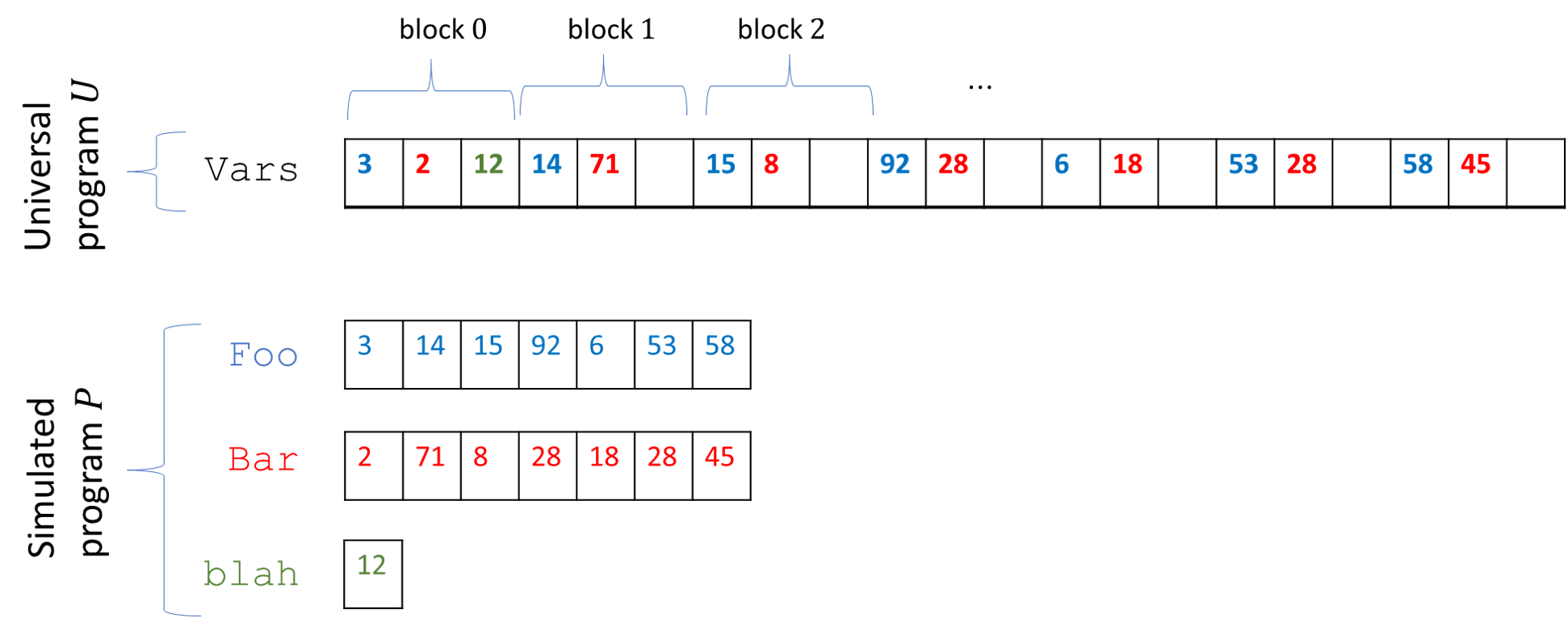
13.5: The universal NAND-RAM program $U$ simulates an input NAND-RAM program $P$ by storing all of $P$’s variables inside a single array `Vars` of $U$. If $P$ has $t$ variables, then the array `Vars` is divided into blocks of length $t$, where the $j$-th coordinate of the $i$-th block contains the $i$-th element of the $j$-th array of $P$. If the $j$-th variable of $P$ is scalar, then we just store its value in the zeroth block of `Vars`.

To present a universal NAND-RAM program in full we would need to describe a precise representation scheme, as well as the full NAND-RAM instructions for the program. While this can be done, it is more important to focus on the main ideas, and so we just sketch the proof here. A specification of NAND-RAM is given in the appendix, and for the purposes of this simulation, we can simply use the representation of the NAND-RAM code as an ASCII string.

The program $U$ gets as input a NAND-RAM program $P$ and an input $x$ and simulates $P$ one step at a time. To do so, $U$ does the following:

$U$ maintains variables program_counter, and number_steps for the current line to be executed and the number of steps executed so far.
$U$ initially scans the code of $P$ to find the number $t$ of unique variable names that $P$ uses. It will translate each variable name into a number between $0$ and $t-1$ and use an array Program to store $P$’s code where for every line $\ell$, Program[$\ell$] will store the $\ell$-th line of $P$ where the variable names have been translated to numbers. (More concretely, we will use a constant number of arrays to separately encode the operation used in this line, and the variable names and indices of the operands.)
$U$ maintains a single array Vars that contains all the values of $P$’s variables. We divide Vars into blocks of length $t$. If $s$ is a number corresponding to an array variable Foo of $P$, then we store Foo[0] in Vars[$s$], we store Foo[1] in Var_values[$t+s$], Foo[2] in Vars[$2t + s$] and so on and so forth (see Figure 13.5). Generally, if the $s$-th variable of $P$ is a scalar variable, then its value will be stored in location Vars[$s$]. If it is an array variable then the value of its $i$-th element will be stored in location Vars[$t\cdot i + s$].
To simulate a single step of $P$, the program $U$ recovers from Program the line corresponding to program_counter and executes it. Since NAND-RAM has a constant number of arithmetic operations, we can implement the logic of which operation to execute using a sequence of a constant number of if-then-else’s. Retrieving from Vars the values of the operands of each instruction can be done using a constant number of arithmetic operations.

The setup stages take only a constant (depending on $|P|$ but not on the input $x$) number of steps. Once we are done with the setup, to simulate a single step of $P$, we just need to retrieve the corresponding line and do a constant number of “if elses” and accesses to Vars to simulate it. Hence the total running time to simulate $T$ steps of the program $P$ is at most $O(T)$ when suppressing constants that depend on the program $P$.

Timed Universal Turing Machine

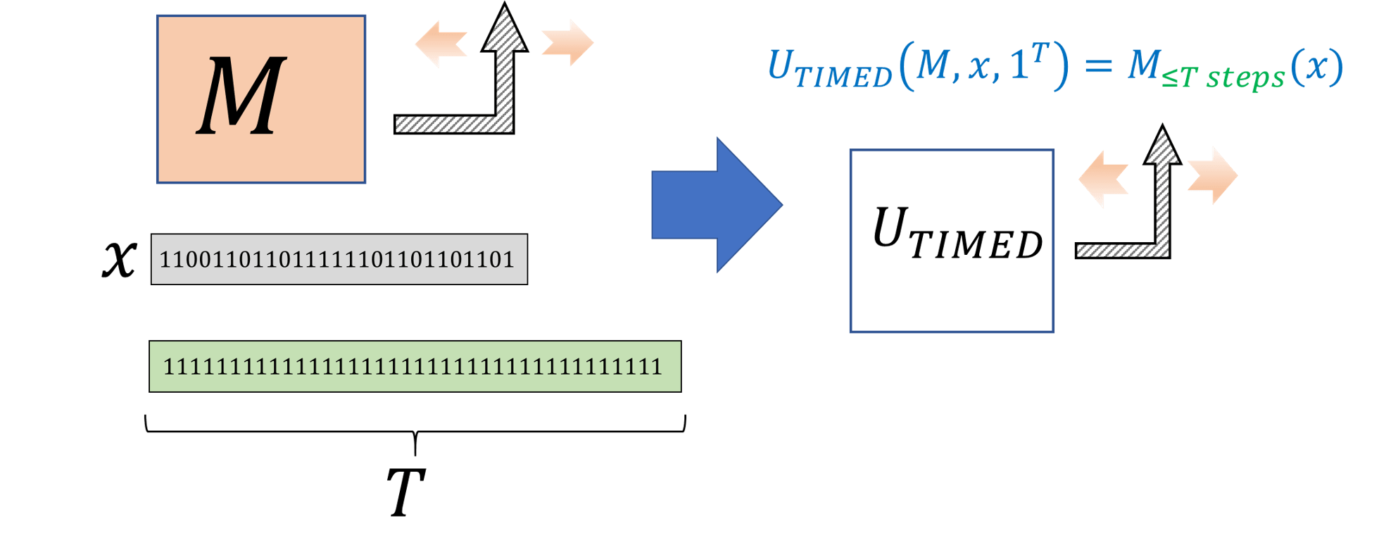
One corollary of the efficient universal machine is the following. Given any Turing machine $M$, input $x$, and “step budget” $T$, we can simulate the execution of $M$ for $T$ steps in time that is polynomial in $T$. Formally, we define a function $\ensuremath{\mathit{TIMEDEVAL}}$ that takes the three parameters $M$, $x$, and the time budget, and outputs $M(x)$ if $M$ halts within at most $T$ steps, and outputs $0$ otherwise. The timed universal Turing machine computes $\ensuremath{\mathit{TIMEDEVAL}}$ in polynomial time (see Figure 13.6). (Since we measure time as a function of the input length, we define $\ensuremath{\mathit{TIMEDEVAL}}$ as taking the input $T$ represented in unary: a string of $T$ ones.)

Let $\ensuremath{\mathit{TIMEDEVAL}}:\{0,1\}^* \rightarrow \{0,1\}^*$ be the function defined as

\[\ensuremath{\mathit{TIMEDEVAL}}(M,x,1^T) = \begin{cases} M(x) & M \text{ halts within $\leq T$ steps on $x$} \\ 0 & \text{otherwise}\end{cases} \;.\]

Then $\ensuremath{\mathit{TIMEDEVAL}} \in \mathbf{P}$.

13.6: The *timed* universal Turing machine takes as input a Turing machine $M$, an input $x$, and a time bound $T$, and outputs $M(x)$ if $M$ halts within at most $T$ steps. Theorem 13.8 states that there is such a machine that runs in time polynomial in $T$.

We only sketch the proof since the result follows fairly directly from Theorem 13.5 and Theorem 13.7. By Theorem 13.5 to show that $\ensuremath{\mathit{TIMEDEVAL}} \in \mathbf{P}$, it suffices to give a polynomial-time NAND-RAM program to compute $\ensuremath{\mathit{TIMEDEVAL}}$.

Such a program can be obtained as follows. Given a Turing machine $M$, by Theorem 13.5 we can transform it in time polynomial in its description into a functionally-equivalent NAND-RAM program $P$ such that the execution of $M$ on $T$ steps can be simulated by the execution of $P$ on $c\cdot T$ steps. We can then run the universal NAND-RAM machine of Theorem 13.7 to simulate $P$ for $c\cdot T$ steps, using $O(T)$ time, and output $0$ if the execution did not halt within this budget. This shows that $\ensuremath{\mathit{TIMEDEVAL}}$ can be computed by a NAND-RAM program in time polynomial in $|M|$ and linear in $T$, which means $\ensuremath{\mathit{TIMEDEVAL}} \in \mathbf{P}$.

The time hierarchy theorem

Some functions are uncomputable, but are there functions that can be computed, but only at an exorbitant cost? For example, is there a function that can be computed in time $2^n$, but can not be computed in time $2^{0.9 n}$? It turns out that the answer is Yes:

For every nice function $T:\N \rightarrow \N$, there is a function $F:\{0,1\}^* \rightarrow \{0,1\}$ in $\ensuremath{\mathit{TIME}}(T(n)\log n) \setminus \ensuremath{\mathit{TIME}}(T(n))$.

There is nothing special about $\log n$, and we could have used any other efficiently computable function that tends to infinity with $n$.

If we have more time, we can compute more functions.

The generality of the time hierarchy theorem can make its proof a little hard to read. It might be easier to follow the proof if you first try to prove by yourself the easier statement $\mathbf{P} \subsetneq \mathbf{EXP}$.

You can do so by showing that the following function $F:\{0,1\}^* :\rightarrow \{0,1\}$ is in $\mathbf{EXP} \setminus \mathbf{P}$: for every Turing machine $M$ and input $x$, $F(M,x)=1$ if and only if $M$ halts on $x$ within at most $|x|^{\log |x|}$ steps. One can show that $F \in \ensuremath{\mathit{TIME}}(n^{O(\log n)}) \subseteq \mathbf{EXP}$ using the universal Turing machine (or the efficient universal NAND-RAM program of Theorem 13.7). On the other hand, we can use similar ideas to those used to show the uncomputability of $\ensuremath{\mathit{HALT}}$ in Section 9.3.2 to prove that $F \not\in \mathbf{P}$.

13.7: The *Time Hierarchy Theorem* (Theorem 13.9) states that all of these classes are *distinct*.

In the proof of Theorem 9.6 (the uncomputability of the Halting problem), we have shown that the function $\ensuremath{\mathit{HALT}}$ cannot be computed in any finite time. An examination of the proof shows that it gives something stronger. Namely, the proof shows that if we fix our computational budget to be $T$ steps, then not only can we not distinguish between programs that halt and those that do not, but we cannot even distinguish between programs that halt within at most $T'$ steps and those that take more than that (where $T'$ is some number depending on $T$). Therefore, the proof of Theorem 13.9 follows the ideas of the uncomputability of the halting problem, but again with a more careful accounting of the running time.

Our proof is inspired by the proof of the uncomputability of the halting problem. Specifically, for every function $T$ as in the theorem’s statement, we define the Bounded Halting function $\ensuremath{\mathit{HALT}}_T$ as follows. The input to $\ensuremath{\mathit{HALT}}_T$ is a pair $(P,x)$ such that $|P| \leq \log \log |x|$ and $P$ encodes some NAND-RAM program. We define

\[ \ensuremath{\mathit{HALT}}_T(P,x) = \begin{cases}1, & P \text{ halts on } x \text{ within } \leq 100\cdot T(|P|+|x|) \text{ steps} \\ 0, & \text{otherwise} \end{cases} \;. \]

(The constant $100$ and the function $\log \log n$ are rather arbitrary, and are chosen for convenience in this proof.)

Theorem 13.9 is an immediate consequence of the following two claims:

Claim 1: $\ensuremath{\mathit{HALT}}_T \in \ensuremath{\mathit{TIME}}(T(n)\cdot \log n)$

and

Claim 2: $\ensuremath{\mathit{HALT}}_T \not\in \ensuremath{\mathit{TIME}}(T(n))$.

Please make sure you understand why indeed the theorem follows directly from the combination of these two claims. We now turn to proving them.

Proof of claim 1: We can easily check in linear time whether an input has the form $P,x$ where $|P| \leq \log\log |x|$. Since $T(\cdot)$ is a nice function, we can evaluate it in $O(T(n))$ time. Thus, we can compute $\ensuremath{\mathit{HALT}}_T(P,x)$ as follows:

Compute $T_0=T(|P|+|x|)$ in $O(T_0)$ steps.
Use the universal NAND-RAM program of Theorem 13.7 to simulate $100\cdot T_0$ steps of $P$ on the input $x$ using at most $poly(|P|)T_0$ steps. (Recall that we use $poly(\ell)$ to denote a quantity that is bounded by $a\ell^b$ for some constants $a,b$.)
If $P$ halts within these $100\cdot T_0$ steps then output $1$, else output $0$.

The length of the input is $n=|P|+|x|$. Since $|x| \leq n$ and $(\log \log |x|)^b = o(\log |x|)$ for every $b$, the running time will be $o(T(|P|+|x|) \log n)$ and hence the above algorithm demonstrates that $\ensuremath{\mathit{HALT}}_T \in \ensuremath{\mathit{TIME}}(T(n)\cdot \log n)$, completing the proof of Claim 1.

Proof of claim 2: This proof is the heart of Theorem 13.9, and is very reminiscent of the proof that $\ensuremath{\mathit{HALT}}$ is not computable. Assume, for the sake of contradiction, that there is some NAND-RAM program $P^*$ that computes $\ensuremath{\mathit{HALT}}_T(P,x)$ within $T(|P|+|x|)$ steps. We are going to show a contradiction by creating a program $Q$ and showing that under our assumptions, if $Q$ runs for less than $T(n)$ steps when given (a padded version of) its own code as input then it actually runs for more than $T(n)$ steps and vice versa. (It is worth re-reading the last sentence twice or thrice to make sure you understand this logic. It is very similar to the direct proof of the uncomputability of the halting problem where we obtained a contradiction by using an assumed “halting solver” to construct a program that, given its own code as input, halts if and only if it does not halt.)

We will define $Q^*$ to be the program that on input a string $z$ does the following:

If $z$ does not have the form $z=P1^m$ where $P$ represents a NAND-RAM program and $|P|< 0.1 \log\log m$ then return $0$. (Recall that $1^m$ denotes the string of $m$ ones.)
Compute $b= P^*(P,z)$ (at a cost of at most $T(|P|+|z|)$ steps, under our assumptions).
If $b=1$ then $Q^*$ goes into an infinite loop, otherwise it halts.

Let $\ell$ be the length description of $Q^*$ as a string, and let $m$ be larger than $2^{2^{1000 \ell}}$. We will reach a contradiction by splitting into cases according to whether or not $\ensuremath{\mathit{HALT}}_T(Q^*,Q^*1^m)$ equals $0$ or $1$.

On the one hand, if $\ensuremath{\mathit{HALT}}_T(Q^*,Q^*1^m)=1$, then under our assumption that $P^*$ computes $\ensuremath{\mathit{HALT}}_T$, $Q^*$ will go into an infinite loop on input $z=Q^*1^m$, and hence in particular $Q^*$ does not halt within $100 T(|Q^*|+m)$ steps on the input $z$. But this contradicts our assumption that $\ensuremath{\mathit{HALT}}_T(Q^*,Q^*1^m)=1$.

This means that it must hold that $\ensuremath{\mathit{HALT}}_T(Q^*,Q^*1^m)=0$. But in this case, since we assume $P^*$ computes $\ensuremath{\mathit{HALT}}_T$, $Q^*$ does not do anything in phase 3 of its computation, and so the only computation costs come in phases 1 and 2 of the computation. It is not hard to verify that Phase 1 can be done in linear and in fact less than $5|z|$ steps. Phase 2 involves executing $P^*$, which under our assumption requires $T(|Q^*|+m)$ steps. In total we can perform both phases in less than $10 T(|Q^*|+m)$ in steps, which by definition means that $\ensuremath{\mathit{HALT}}_T(Q^*,Q^*1^m)=1$, but this is of course a contradiction. This completes the proof of Claim 2 and hence of Theorem 13.9.

Prove that $\mathbf{P} \subsetneq \mathbf{EXP}$.

This statement follows directly from the time hierarchy theorem, but it can be an instructive exercise to prove it directly, see Remark 13.10. We need to show that there exists $F \in \mathbf{EXP} \setminus \mathbf{P}$. Let $T(n) = n^{\log n}$ and $T'(n) = n^{\log n / 2}$. Both are nice functions. Since $T(n)/T'(n) = \omega(\log n)$, by Theorem 13.9 there exists some $F$ in $\ensuremath{\mathit{TIME}}(T(n)) \setminus \ensuremath{\mathit{TIME}}(T'(n))$. Since for sufficiently large $n$, $2^n > n^{\log n}$, $F \in \ensuremath{\mathit{TIME}}(2^n) \subseteq \mathbf{EXP}$. On the other hand, $F \not\in \mathbf{P}$. Indeed, suppose otherwise that there was a constant $c>0$ and a Turing machine computing $F$ on $n$-length input in at most $n^c$ steps for all sufficiently large $n$. Then since for $n$ large enough $n^c < n^{\log n/2}$, it would have followed that $F \in \ensuremath{\mathit{TIME}}(n^{\log n /2})$ contradicting our choice of $F$.

The time hierarchy theorem tells us that there are functions we can compute in $O(n^2)$ time but not $O(n)$, in $2^n$ time, but not $2^{\sqrt{n}}$, etc.. In particular there are most definitely functions that we can compute in time $2^n$ but not $O(n)$. We have seen that we have no shortage of natural functions for which the best known algorithm requires roughly $2^n$ time, and that many people have invested significant effort in trying to improve that. However, unlike in the finite vs. infinite case, for all of the examples above at the moment we do not know how to rule out even an $O(n)$ time algorithm. We will however see that there is a single unproven conjecture that would imply such a result for most of these problems.

13.8: Some complexity classes and some of the functions we know (or conjecture) to be contained in them.

The time hierarchy theorem relies on the existence of an efficient universal NAND-RAM program, as proven in Theorem 13.7. For other models such as Turing machines we have similar time hierarchy results showing that there are functions computable in time $T(n)$ and not in time $T(n)/f(n)$ where $f(n)$ corresponds to the overhead in the corresponding universal machine.

Non-uniform computation

We have now seen two measures of “computation cost” for functions. In Section 4.6 we defined the complexity of computing finite functions using circuits / straightline programs. Specifically, for a finite function $g:\{0,1\}^n \rightarrow \{0,1\}$ and number $s\in \N$, $g\in \ensuremath{\mathit{SIZE}}_n(s)$ if there is a circuit of at most $s$ NAND gates (or equivalently an $s$-line NAND-CIRC program) that computes $g$. To relate this to the classes $\ensuremath{\mathit{TIME}}(T(n))$ defined in this chapter we first need to extend the class $\ensuremath{\mathit{SIZE}}_n(s)$ from finite functions to functions with unbounded input length.

Let $F:\{0,1\}^* \rightarrow \{0,1\}$ and $T:\N \rightarrow \N$ be a nice time bound. For every $n\in \N$, define $F_{\upharpoonright n} : \{0,1\}^n \rightarrow \{0,1\}$ to be the restriction of $F$ to inputs of size $n$. That is, $F_{\upharpoonright n}$ is the function mapping $\{0,1\}^n$ to $\{0,1\}$ such that for every $x\in \{0,1\}^n$, $F_{\upharpoonright n}(x)=F(x)$.

We say that $F$ is non-uniformly computable in at most $T(n)$ size, denoted by $F \in \ensuremath{\mathit{SIZE}}(T)$ if there exists a sequence $(C_0,C_1,C_2,\ldots)$ of NAND circuits such that:

For every $n\in \N$, $C_n$ computes the function $F_{\upharpoonright n}$
For every sufficiently large $n$, $C_n$ has at most $T(n)$ gates.

In other words, $F \in \ensuremath{\mathit{SIZE}}(T)$ iff for every $n \in \N$, it holds that $F_{\upharpoonright n} \in \ensuremath{\mathit{SIZE}}_n(T(n))$. The non-uniform analog to the class $\mathbf{P}$ is the class $\mathbf{P_{/poly}}$ defined as

\[ \mathbf{P_{/poly}} = \cup_{c\in \N} \ensuremath{\mathit{SIZE}}(n^c) \; . \;\;(13.2) \]

There is a big difference between non-uniform computation and uniform complexity classes such as $\ensuremath{\mathit{TIME}}(T(n))$ or $\mathbf{P}$. The condition $F\in \mathbf{P}$ means that there is a single Turing machine $M$ that computes $F$ on all inputs in polynomial time. The condition $F\in \mathbf{P_{/poly}}$ only means that for every input length $n$ there can be a different circuit $C_n$ that computes $F$ using polynomially many gates on inputs of these lengths. As we will see, $F\in \mathbf{P_{/poly}}$ does not necessarily imply that $F\in \mathbf{P}$. However, the other direction is true:

13.9: We can think of an infinite function $F:\{0,1\}^* \rightarrow \{0,1\}$ as a collection of finite functions $F_0,F_1,F_2,\ldots$ where $F_{\upharpoonright n}:\{0,1\}^n \rightarrow \{0,1\}$ is the restriction of $F$ to inputs of length $n$. We say $F$ is in $\mathbf{P_{/poly}}$ if for every $n$, the function $F_{\upharpoonright n}$ is computable by a polynomial-size NAND-CIRC program, or equivalently, a polynomial-sized Boolean circuit.

There is some $a\in \N$ s.t. for every nice $T:\N \rightarrow \N$ and $F:\{0,1\}^* \rightarrow \{0,1\}$,

\[\ensuremath{\mathit{TIME}}(T(n)) \subseteq \ensuremath{\mathit{SIZE}}(T(n)^a)\;.\]

In particular, Theorem 13.12 shows that for every $c$, $\ensuremath{\mathit{TIME}}(n^c) \subseteq \ensuremath{\mathit{SIZE}}(n^{ca})$ and hence $\mathbf{P} \subseteq \mathbf{P_{/poly}}$.

The idea behind the proof is to “unroll the loop”. Specifically, we will use the programming language variants of non-uniform and uniform computation: namely NAND-CIRC and NAND-TM. The main difference between the two is that NAND-TM has loops. However, for every fixed $n$, if we know that a NAND-TM program runs in at most $T(n)$ steps, then we can replace its loop by simply “copying and pasting” its code $T(n)$ times, similar to how in Python we can replace code such as

for i in range(4):
    print(i)

with the “loop free” code

print(0)
print(1)
print(2)
print(3)

To make this idea into an actual proof we need to tackle one technical difficulty, and this is to ensure that the NAND-TM program is oblivious in the sense that the value of the index variable i in the $j$-th iteration of the loop will depend only on $j$ and not on the contents of the input. We make a digression to do just that in Section 13.6.1 and then complete the proof of Theorem 13.12.

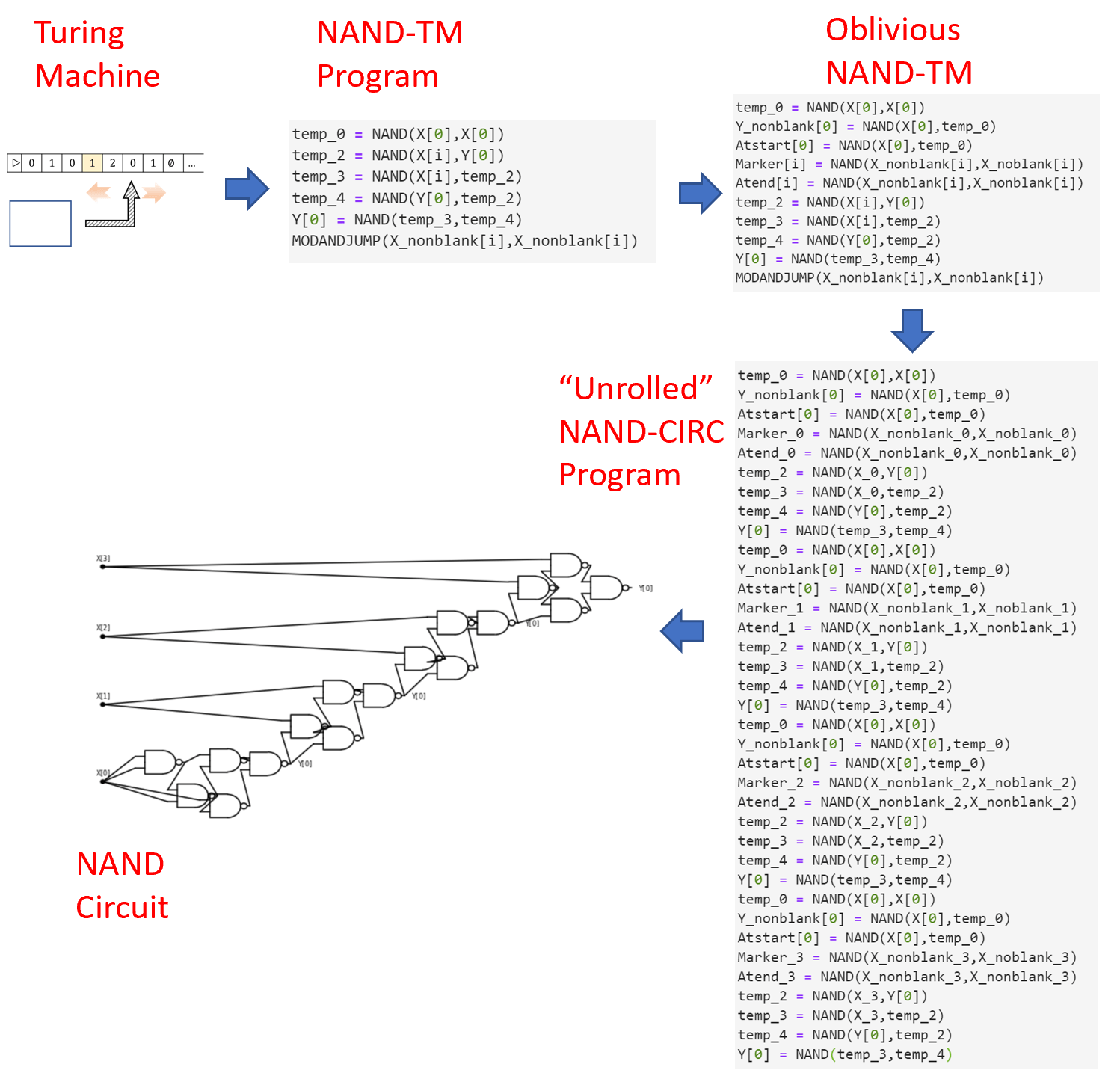
Oblivious NAND-TM programs

Our approach for proving Theorem 13.12 involves “unrolling the loop”. For example, consider the following NAND-TM to compute the $\ensuremath{\mathit{XOR}}$ function on inputs of arbitrary length:

temp_0 = NAND(X[0],X[0])
Y_nonblank[0] = NAND(X[0],temp_0)
temp_2 = NAND(X[i],Y[0])
temp_3 = NAND(X[i],temp_2)
temp_4 = NAND(Y[0],temp_2)
Y[0] = NAND(temp_3,temp_4)
MODANDJUMP(X_nonblank[i],X_nonblank[i])

Setting (as an example) $n=3$, we can attempt to translate this NAND-TM program into a NAND-CIRC program for computing $\ensuremath{\mathit{XOR}}_3:\{0,1\}^3 \rightarrow \{0,1\}$ by simply “copying and pasting” the loop three times (dropping the MODANDJMP line):

temp_0 = NAND(X[0],X[0])
Y_nonblank[0] = NAND(X[0],temp_0)
temp_2 = NAND(X[i],Y[0])
temp_3 = NAND(X[i],temp_2)
temp_4 = NAND(Y[0],temp_2)
Y[0] = NAND(temp_3,temp_4)
temp_0 = NAND(X[0],X[0])
Y_nonblank[0] = NAND(X[0],temp_0)
temp_2 = NAND(X[i],Y[0])
temp_3 = NAND(X[i],temp_2)
temp_4 = NAND(Y[0],temp_2)
Y[0] = NAND(temp_3,temp_4)
temp_0 = NAND(X[0],X[0])
Y_nonblank[0] = NAND(X[0],temp_0)
temp_2 = NAND(X[i],Y[0])
temp_3 = NAND(X[i],temp_2)
temp_4 = NAND(Y[0],temp_2)
Y[0] = NAND(temp_3,temp_4)

However, the above is still not a valid NAND-CIRC program since it contains references to the special variable i. To make it into a valid NAND-CIRC program, we replace references to i in the first iteration with $0$, references in the second iteration with $1$, and references in the third iteration with $2$. (We also create a variable zero and use it for the first time any variable is instantiated, as well as remove assignments to non-output variables that are never used later on.) The resulting program is a standard “loop free and index free” NAND-CIRC program that computes $\ensuremath{\mathit{XOR}}_3$ (see also Figure 13.10):

temp_0 = NAND(X[0],X[0])
one = NAND(X[0],temp_0)
zero = NAND(one,one)
temp_2 = NAND(X[0],zero)
temp_3 = NAND(X[0],temp_2)
temp_4 = NAND(zero,temp_2)
Y[0] = NAND(temp_3,temp_4)
temp_2 = NAND(X[1],Y[0])
temp_3 = NAND(X[1],temp_2)
temp_4 = NAND(Y[0],temp_2)
Y[0] = NAND(temp_3,temp_4)
temp_2 = NAND(X[2],Y[0])
temp_3 = NAND(X[2],temp_2)
temp_4 = NAND(Y[0],temp_2)
Y[0] = NAND(temp_3,temp_4)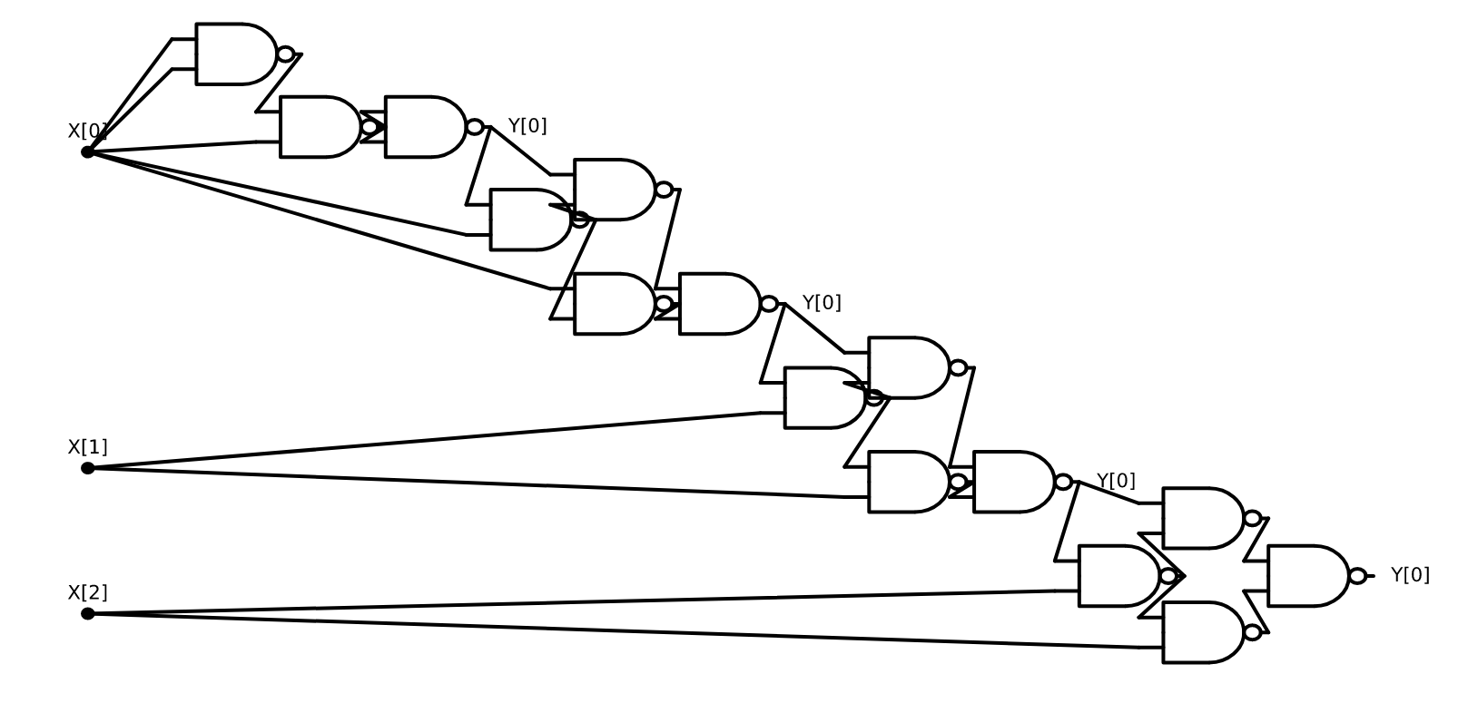

13.10: A NAND circuit for $\ensuremath{\mathit{XOR}}_3$ obtained by “unrolling the loop” of the NAND-TM program for computing $\ensuremath{\mathit{XOR}}$ three times.

Key to this transformation was the fact that in our original NAND-TM program for $\ensuremath{\mathit{XOR}}$, regardless of whether the input is $011$, $100$, or any other string, the index variable i is guaranteed to equal $0$ in the first iteration, $1$ in the second iteration, $2$ in the third iteration, and so on and so forth. The particular sequence $0,1,2,\ldots$ is immaterial: the crucial property is that the NAND-TM program for $\ensuremath{\mathit{XOR}}$ is oblivious in the sense that the value of the index i in the $j$-th iteration depends only on $j$ and does not depend on the particular choice of the input. Luckily, it is possible to transform every NAND-TM program into a functionally equivalent oblivious program with at most quadratic overhead. (Similarly we can transform any Turing machine into a functionally equivalent oblivious Turing machine, see Exercise 13.6.)

Let $T:\N \rightarrow \N$ be a nice function and let $F\in \ensuremath{\mathit{TIME}}_{\mathsf{TM}}(T(n))$. Then there is a NAND-TM program $P$ that computes $F$ in $O(T(n)^2)$ steps and satisfying the following. For every $n\in \N$ there is a sequence $i_0,i_1,\ldots, i_{m-1}$ such that for every $x\in \{0,1\}^n$, if $P$ is executed on input $x$ then in the $j$-th iteration the variable i is equal to $i_j$.

In other words, Theorem 13.13 implies that if we can compute $F$ in $T(n)$ steps, then we can compute it in $O(T(n)^2)$ steps with a program $P$ in which the position of i in the $j$-th iteration depends only on $j$ and the length of the input, and not on the contents of the input. Such a program can be easily translated into a NAND-CIRC program of $O(T(n)^2)$ lines by “unrolling the loop”.

We can translate any NAND-TM program $P'$ into an oblivious program $P$ by making $P$ “sweep” its arrays. That is, the index i in $P$ will always move all the way from position $0$ to position $T(n)-1$ and back again. We can then simulate the program $P'$ with at most $T(n)$ overhead: if $P'$ wants to move i left when we are in a rightward sweep then we simply wait the at most $2T(n)$ steps until the next time we are back in the same position while sweeping to the left.

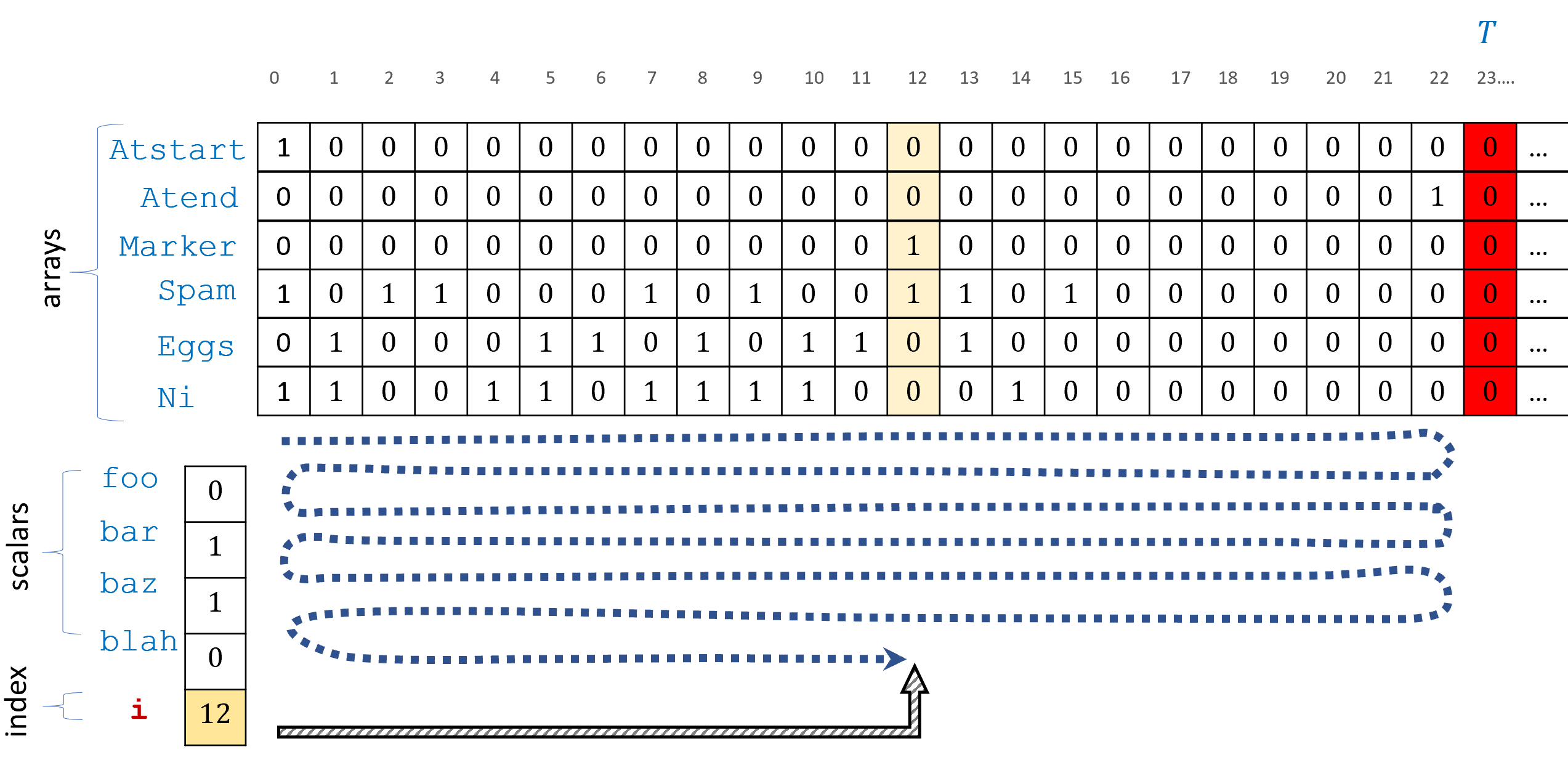
13.11: We simulate a $T(n)$-time NAND-TM program $P'$ with an *oblivious* NAND-TM program $P$ by adding special arrays `Atstart` and `Atend` to mark positions $0$ and $T-1$ respectively. The program $P$ will simply “sweep” its arrays from right to left and back again. If the original program $P'$ would have moved `i` in a different direction then we wait $O(T)$ steps until we reach the same point back again, and so $P$ runs in $O(T(n)^2)$ time.

Let $P'$ be a NAND-TM program computing $F$ in $T(n)$ steps. We construct an oblivious NAND-TM program $P$ for computing $F$ as follows (see also Figure 13.11).

On input $x$, $P$ will compute $T=T(|x|)$ and set up arrays Atstart and Atend satisfying Atstart[$0$]$=1$ and Atstart[$i$]$=0$ for $i>0$ and Atend[$T-1$]$=1$ and Atend[i]$=0$ for all $i \neq T-1$. We can do this because $T$ is a nice function. Note that since this computation does not depend on $x$ but only on its length, it is oblivious.
$P$ will also have a special array Marker initialized to all zeroes.
The index variable of $P$ will change direction of movement to the right whenever Atstart[i]$=1$ and to the left whenever Atend[i]$=1$.
The program $P$ simulates the execution of $P'$. However, if the MODANDJMP instruction in $P'$ attempts to move to the right when $P$ is moving left (or vice versa) then $P$ will set Marker[i] to $1$ and enter into a special “waiting mode”. In this mode $P$ will wait until the next time in which Marker[i]$=1$ (at the next sweep) at which points $P$ zeroes Marker[i] and continues with the simulation. In the worst case this will take $2T(n)$ steps (if $P$ has to go all the way from one end to the other and back again.)
We also modify $P$ to ensure it ends the computation after simulating exactly $T(n)$ steps of $P'$, adding “dummy steps” if $P'$ ends early.

We see that $P$ simulates the execution of $P'$ with an overhead of $O(T(n))$ steps of $P$ per one step of $P'$, hence completing the proof.

Theorem 13.13 implies Theorem 13.12. Indeed, if $P$ is a $k$-line oblivious NAND-TM program computing $F$ in time $T(n)$ then for every $n$ we can obtain a NAND-CIRC program of $(k-1)\cdot T(n)$ lines by simply making $T(n)$ copies of $P$ (dropping the final MODANDJMP line). In the $j$-th copy we replace all references of the form Foo[i] to foo_$i_j$ where $i_j$ is the value of i in the $j$-th iteration.

“Unrolling the loop”: algorithmic transformation of Turing Machines to circuits

The proof of Theorem 13.12 is algorithmic, in the sense that the proof yields a polynomial-time algorithm that given a Turing machine $M$ and parameters $T$ and $n$, produces a circuit of $O(T^2)$ gates that agrees with $M$ on all inputs $x\in \{0,1\}^n$ (as long as $M$ runs for less than $T$ steps these inputs.) We record this fact in the following theorem, since it will be useful for us later on:

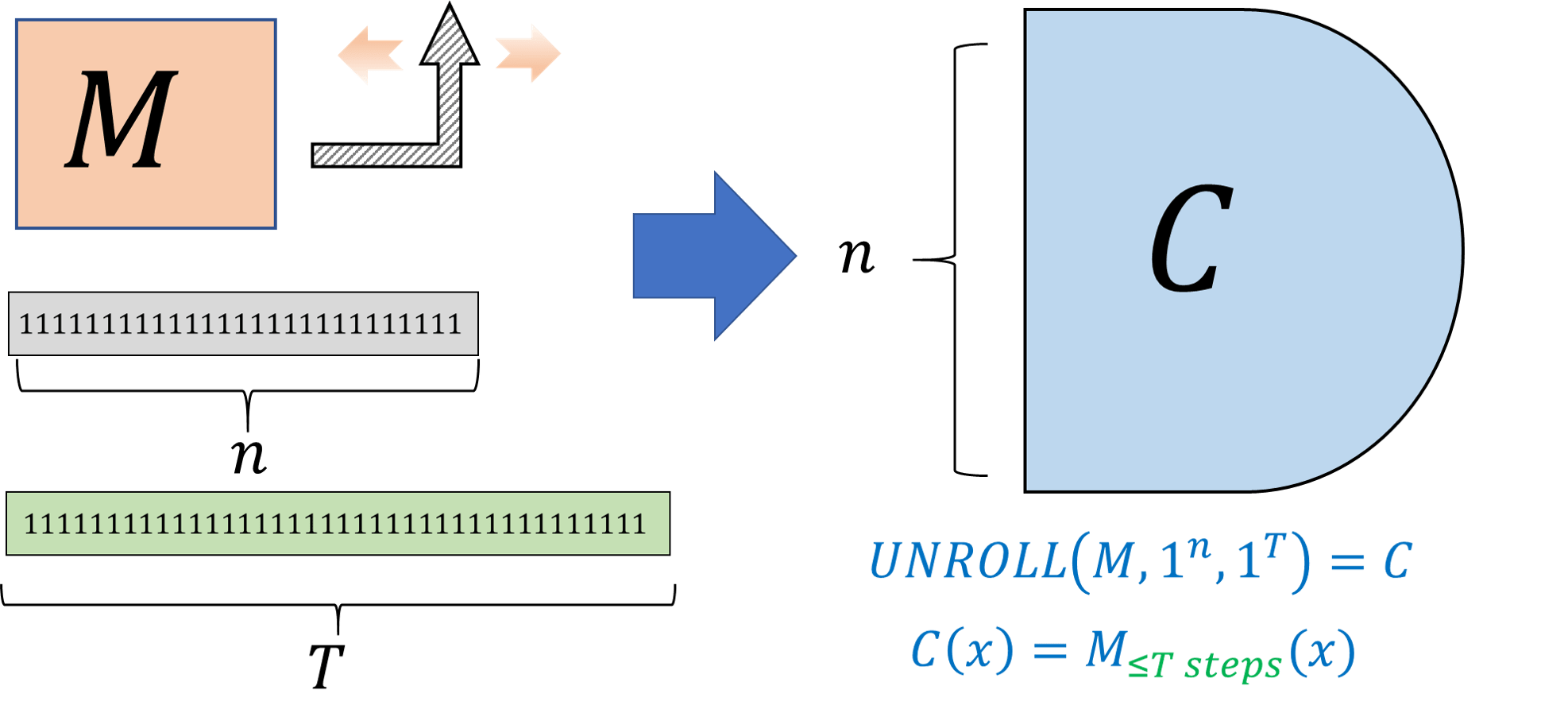
13.12: The function $\ensuremath{\mathit{UNROLL}}$ takes as input a Turing machine $M$, an input length parameter $n$, a step budget parameter $T$, and outputs a circuit $C$ of size $poly(T)$ that takes $n$ bits of inputs and outputs $M(x)$ if $M$ halts on $x$ within at most $T$ steps.

There is algorithm $\ensuremath{\mathit{UNROLL}}$ such that for every Turing machine $M$ and numbers $n,T$, $\ensuremath{\mathit{UNROLL}}(M,1^T,1^n)$ runs for $poly(|M|,T,n)$ steps and outputs a NAND circuit $C$ with $n$ inputs, $O(T^2)$ gates, and one output, such that

\[ C(x) = \begin{cases}y & M \text{ halts in $\leq T$ steps and outputs $y$} \\ 0 & \text{otherwise} \end{cases}\;. \]

We only sketch the proof since it follows by directly translating the proof of Theorem 13.12 into an algorithm together with the simulation of Turing machines by NAND-TM programs (see also Figure 13.13). Specifically, $\ensuremath{\mathit{UNROLL}}$ does the following:

Transform the Turing machine $M$ into an equivalent NAND-TM program $P$.
Transform the NAND-TM program $P$ into an equivalent oblivious program $P'$ following the proof of Theorem 13.13. The program $P'$ takes $T' = O(T^2)$ steps to simulate $T$ steps of $P$.
“Unroll the loop” of $P'$ by obtaining a NAND-CIRC program of $O(T')$ lines (or equivalently a NAND circuit with $O(T^2)$ gates) corresponding to the execution of $T'$ iterations of $P'$.

13.13: We can transform a Turing machine $M$, input length parameter $n$, and time bound $T$ into an $O(T^2)$-sized NAND circuit that agrees with $M$ on all inputs $x\in \{0,1\}^n$ on which $M$ halts in at most $T$ steps. The transformation is obtained by first using the equivalence of Turing machines and NAND-TM programs $P$, then turning $P$ into an equivalent *oblivious* NAND-TM program $P'$ via Theorem 13.13, then “unrolling” $O(T^2)$ iterations of the loop of $P'$ to obtain an $O(T^2)$ line NAND-CIRC program that agrees with $P'$ on length $n$ inputs, and finally translating this program into an equivalent circuit.

By “unrolling the loop” we can transform an algorithm that takes $T(n)$ steps to compute $F$ into a circuit that uses $poly(T(n))$ gates to compute the restriction of $F$ to $\{0,1\}^n$.

Reviewing the transformations described in Figure 13.13, as well as solving the following two exercises is a great way to get more comfort with non-uniform complexity and in particular with $\mathbf{P_{/poly}}$ and its relation to $\mathbf{P}$.

Prove that for every $F:\{0,1\}^* \rightarrow \{0,1\}$, $F\in \mathbf{P}$ if and only if there is a polynomial-time Turing machine $M$ such that for every $n\in \N$, $M(1^n)$ outputs a description of an $n$ input circuit $C_n$ that computes the restriction $F_{\upharpoonright n}$ of $F$ to inputs in $\{0,1\}^n$.

We start with the “if” direction. Suppose that there is a polynomial-time Turing machine $M$ that on input $1^n$ outputs a circuit $C_n$ that computes $F_{\upharpoonright n}$. Then the following is a polynomial-time Turing machine $M'$ to compute $F$. On input $x\in \{0,1\}^*$, $M'$ will:

Let $n=|x|$ and compute $C_n = M(1^n)$.
Return the evaluation of $C_n$ on $x$.

Since we can evaluate a Boolean circuit on an input in polynomial time, $M'$ runs in polynomial time and computes $F(x)$ on every input $x$.

For the “only if” direction, if $M'$ is a Turing machine that computes $F$ in polynomial-time, then (applying the equivalence of Turing machines and NAND-TM as well as Theorem 13.13) there is also an oblivious NAND-TM program $P$ that computes $F$ in time $p(n)$ for some polynomial $p$. We can now define $M$ to be the Turing machine that on input $1^n$ outputs the NAND circuit obtained by “unrolling the loop” of $P$ for $p(n)$ iterations. The resulting NAND circuit computes $F_{\upharpoonright n}$ and has $O(p(n))$ gates. It can also be transformed to a Boolean circuit with $O(p(n))$ AND/OR/NOT gates.

Let $F:\{0,1\}^* \rightarrow \{0,1\}$. Then $F\in\mathbf{P_{/poly}}$ if and only if there exists a polynomial $p:\N \rightarrow \N$, a polynomial-time Turing machine $M$ and a sequence $\{ a_n \}_{n\in \N}$ of strings, such that for every $n\in \N$:

$|a_n| \leq p(n)$
For every $x\in \{0,1\}^n$, $M(a_n,x)=F(x)$.

We only sketch the proof. For the “only if” direction, if $F\in \mathbf{P_{/poly}}$ then we can use for $a_n$ simply the description of the corresponding circuit $C_n$ and for $M$ the program that computes in polynomial time the evaluation of a circuit on its input.

For the “if” direction, we can use the same “unrolling the loop” technique of Theorem 13.12 to show that if $P$ is a polynomial-time NAND-TM program, then for every $n\in \N$, the map $x \mapsto P(a_n,x)$ can be computed by a polynomial-size NAND-CIRC program $Q_n$.

Can uniform algorithms simulate non-uniform ones?

Theorem 13.12 shows that every function in $\ensuremath{\mathit{TIME}}(T(n))$ is in $\ensuremath{\mathit{SIZE}}(poly(T(n)))$. One can ask if there is an inverse relation. Suppose that $F$ is such that $F_{\upharpoonright n}$ has a “short” NAND-CIRC program for every $n$. Can we say that it must be in $\ensuremath{\mathit{TIME}}(T(n))$ for some “small” $T$? The answer is an emphatic no. Not only is $\mathbf{P_{/poly}}$ not contained in $\mathbf{P}$, in fact $\mathbf{P_{/poly}}$ contains functions that are uncomputable!

There exists an uncomputable function $F:\{0,1\}^* \rightarrow \{0,1\}$ such that $F \in \mathbf{P_{/poly}}$.

Since $\mathbf{P_{/poly}}$ corresponds to non-uniform computation, a function $F$ is in $\mathbf{P_{/poly}}$ if for every $n\in \N$, the restriction $F_{\upharpoonright n}$ to inputs of length $n$ has a small circuit/program, even if the circuits for different values of $n$ are completely different from one another. In particular, if $F$ has the property that for every equal-length inputs $x$ and $x'$, $F(x)=F(x')$ then this means that $F_{\upharpoonright n}$ is either the constant function zero or the constant function one for every $n\in \N$. Since the constant function has a (very!) small circuit, such a function $F$ will always be in $\mathbf{P_{/poly}}$ (indeed even in smaller classes). Yet by a reduction from the Halting problem, we can obtain a function with this property that is uncomputable.

Consider the following “unary halting function” $\ensuremath{\mathit{UH}}:\{0,1\}^* \rightarrow \{0,1\}$ defined as follows. We let $S:\N \rightarrow \{0,1\}^*$ be the function that on input $n\in \N$, outputs the string that corresponds to the binary representation of the number $n$ without the most significant $1$ digit. Note that $S$ is onto. For every $x\in \{0,1\}^*$, we define $\ensuremath{\mathit{UH}}(x)=\ensuremath{\mathit{HALTONZERO}}(S(|x|))$. That is, if $n$ is the length of $x$, then $\ensuremath{\mathit{UH}}(x)=1$ if and only if the string $S(n)$ encodes a NAND-TM program that halts on the input $0$.

$\ensuremath{\mathit{UH}}$ is uncomputable, since otherwise we could compute $\ensuremath{\mathit{HALTONZERO}}$ by transforming the input program $P$ into the integer $n$ such that $P=S(n)$ and then running $\ensuremath{\mathit{UH}}(1^n)$ (i.e., $\ensuremath{\mathit{UH}}$ on the string of $n$ ones). On the other hand, for every $n$, $\ensuremath{\mathit{UH}}_n(x)$ is either equal to $0$ for all inputs $x$ or equal to $1$ on all inputs $x$, and hence can be computed by a NAND-CIRC program of a constant number of lines.

The issue here is of course uniformity. For a function $F:\{0,1\}^* \rightarrow \{0,1\}$, if $F$ is in $\ensuremath{\mathit{TIME}}(T(n))$ then we have a single algorithm that can compute $F_{\upharpoonright n}$ for every $n$. On the other hand, $F_{\upharpoonright n}$ might be in $\ensuremath{\mathit{SIZE}}(T(n))$ for every $n$ using a completely different algorithm for every input length. For this reason we typically use $\mathbf{P_{/poly}}$ not as a model of efficient computation but rather as a way to model inefficient computation. For example, in cryptography people often define an encryption scheme to be secure if breaking it for a key of length $n$ requires more than a polynomial number of NAND lines. Since $\mathbf{P} \subseteq \mathbf{P_{/poly}}$, this in particular precludes a polynomial time algorithm for doing so, but there are technical reasons why working in a non-uniform model makes more sense in cryptography. It also allows to talk about security in non-asymptotic terms such as a scheme having “$128$ bits of security”.

While it can sometimes be a real issue, in many natural settings the difference between uniform and non-uniform computation does not seem so important. In particular, in all the examples of problems not known to be in $\mathbf{P}$ we discussed before: longest path, 3SAT, factoring, etc., these problems are also not known to be in $\mathbf{P_{/poly}}$ either. Thus, for “natural” functions, if you pretend that $\ensuremath{\mathit{TIME}}(T(n))$ is roughly the same as $\ensuremath{\mathit{SIZE}}(T(n))$, you will be right more often than wrong.

13.14: Relations between $\mathbf{P}$, $\mathbf{EXP}$, and $\mathbf{P_{/poly}}$. It is known that $\mathbf{P} \subseteq \mathbf{EXP}$, $\mathbf{P} \subseteq \mathbf{P_{/poly}}$ and that $\mathbf{P_{/poly}}$ contains uncomputable functions (which in particular are outside of $\mathbf{EXP}$). It is not known whether or not $\mathbf{EXP} \subseteq \mathbf{P_{/poly}}$ though it is believed that $\mathbf{EXP} \not\subseteq \mathbf{P_{/poly}}$.

Uniform vs. Non-uniform computation: A recap

To summarize, the two models of computation we have described so far are:

Uniform models: Turing machines, NAND-TM programs, RAM machines, NAND-RAM programs, C/JavaScript/Python, etc. These models include loops and unbounded memory hence a single program can compute a function with unbounded input length.
Non-uniform models: Boolean Circuits or straightline programs have no loops and can only compute finite functions. The time to execute them is exactly the number of lines or gates they contain.

For a function $F:\{0,1\}^* \rightarrow \{0,1\}$ and some nice time bound $T:\N \rightarrow \N$, we know that:

If $F$ is uniformly computable in time $T(n)$ then there is a sequence of circuits $C_1,C_2,\ldots$ where $C_n$ has $poly(T(n))$ gates and computes $F_{\upharpoonright n}$ (i.e., restriction of $F$ to $\{0,1\}^n$) for every $n$.
The reverse direction is not necessarily true - there are examples of functions $F:\{0,1\}^n \rightarrow \{0,1\}$ such that $F_{\upharpoonright n}$ can be computed by even a constant size circuit but $F$ is uncomputable.

This means that non-uniform complexity is more useful to establish hardness of a function than its easiness.

We can define the time complexity of a function using NAND-TM programs, and similarly to the notion of computability, this appears to capture the inherent complexity of the function.
There are many natural problems that have polynomial-time algorithms, and other natural problems that we’d love to solve, but for which the best known algorithms are exponential.
The definition of polynomial time, and hence the class $\mathbf{P}$, is robust to the choice of model, whether it is Turing machines, NAND-TM, NAND-RAM, modern programming languages, and many other models.
The time hierarchy theorem shows that there are some problems that can be solved in exponential, but not in polynomial time. However, we do not know if that is the case for the natural examples that we described in this lecture.
By “unrolling the loop” we can show that every function computable in time $T(n)$ can be computed by a sequence of NAND-CIRC programs (one for every input length) each of size at most $poly(T(n))$.

Exercises

Prove that the classes $\mathbf{P}$ and $\mathbf{EXP}$ defined in Definition 13.2 are equal to $\cup_{c\in \{1,2,3,\ldots \}} \ensuremath{\mathit{TIME}}(n^c)$ and $\cup_{c\in \{1,2,3,\ldots \}} \ensuremath{\mathit{TIME}}(2^{n^c})$ respectively. (If $S_1,S_2,S_3,\ldots$ is a collection of sets then the set $S = \cup_{c\in \{1,2,3,\ldots \}} S_c$ is the set of all elements $e$ such that there exists some $c\in \{ 1,2,3,\ldots \}$ where $e\in S_c$.)

Theorem 13.5 shows that the classes $\mathbf{P}$ and $\mathbf{EXP}$ are robust with respect to variations in the choice of the computational model. This exercise shows that these classes are also robust with respect to our choice of the representation of the input.

Specifically, let $F$ be a function mapping graphs to $\{0,1\}$, and let $F', F'':\{0,1\}^* \rightarrow \{0,1\}$ be the functions defined as follows. For every $x\in \{0,1\}^*$:

$F'(x)=1$ iff $x$ represents a graph $G$ via the adjacency matrix representation such that $F(G)=1$.
$F''(x)=1$ iff $x$ represents a graph $G$ via the adjacency list representation such that $F(G)=1$.

Prove that $F' \in \mathbf{P}$ iff $F'' \in \mathbf{P}$.

More generally, for every function $F:\{0,1\}^* \rightarrow \{0,1\}$, the answer to the question of whether $F\in \mathbf{P}$ (or whether $F\in \mathbf{EXP}$) is unchanged by switching representations, as long as transforming one representation to the other can be done in polynomial time (which essentially holds for all reasonable representations).

For every function $F:\{0,1\}^* \rightarrow \{0,1\}^*$, define $Bool(F)$ to be the function mapping $\{0,1\}^*$ to $\{0,1\}$ such that on input a (string representation of a) triple $(x,i,\sigma)$ with $x\in \{0,1\}^*$, $i \in \N$ and $\sigma \in \{0,1\}$,

\[ Bool(F)(x,i,\sigma) = \begin{cases} F(x)_i & \sigma =0, i<|F(x)| \\ 1 & \sigma = 1,i<|F(x)| \\ 0 & \text{otherwise} \end{cases} \]

where $F(x)_i$ is the $i$-th bit of the string $F(x)$.

Prove that for every $F:\{0,1\}^* \rightarrow \{0,1\}^*$, $Bool(F) \in \mathbf{P}$ if and only if there is a Turing Machine $M$ and a polynomial $p:\N \rightarrow \N$ such that for every $x\in \{0,1\}^*$, on input $x$, $M$ halts within $\leq p(|x|)$ steps and outputs $F(x)$.

Say that a (possibly non-Boolean) function $F:\{0,1\}^* \rightarrow \{0,1\}^*$ is computable in polynomial time, if there is a Turing Machine $M$ and a polynomial $p:\N \rightarrow \N$ such that for every $x\in \{0,1\}^*$, on input $x$, $M$ halts within $\leq p(|x|)$ steps and outputs $F(x)$. Prove that for every pair of functions $F,G:\{0,1\}^* \rightarrow \{0,1\}^*$ computable in polynomial time, their composition $F\circ G$, which is the function $H$ s.t. $H(x)=F(G(x))$, is also computable in polynomial time.

Say that a (possibly non-Boolean) function $F:\{0,1\}^* \rightarrow \{0,1\}^*$ is computable in exponential time, if there is a Turing Machine $M$ and a polynomial $p:\N \rightarrow \N$ such that for every $x\in \{0,1\}^*$, on input $x$, $M$ halts within $\leq 2^{p(|x|)}$ steps and outputs $F(x)$. Prove that there is some $F,G:\{0,1\}^* \rightarrow \{0,1\}^*$ s.t. both $F$ and $G$ are computable in exponential time, but $F\circ G$ is not computable in exponential time.

We say that a Turing machine $M$ is oblivious if there is some function $T:\N\times \N \rightarrow \Z$ such that for every input $x$ of length $n$, and $t\in \N$ it holds that:

If $M$ takes more than $t$ steps to halt on the input $x$, then in the $t$-th step $M$’s head will be in the position $T(n,t)$. (Note that this position depends only on the length of $x$ and not its contents.)
If $M$ halts before the $t$-th step then $T(n,t) = -1$.

Prove that if $F\in \mathbf{P}$ then there exists an oblivious Turing machine $M$ that computes $F$ in polynomial time. See footnote for hint.¹

Let $\ensuremath{\mathit{EDGE}}:\{0,1\}^* \rightarrow \{0,1\}$ be the function such that on input a string representing a triple $(L,i,j)$, where $L$ is the adjacency list representation of an $n$ vertex graph $G$, and $i$ and $j$ are numbers in $[n]$, $\ensuremath{\mathit{EDGE}}(L,i,j)=1$ if the edge $\{i,j \}$ is present in the graph. $\ensuremath{\mathit{EDGE}}$ outputs $0$ on all other inputs.

Prove that $\ensuremath{\mathit{EDGE}} \in \mathbf{P}$.
Let $\ensuremath{\mathit{PLANARMATRIX}}:\{0,1\}^* \rightarrow \{0,1\}$ be the function that on input an adjacency matrix $A$ outputs $1$ if and only if the graph represented by $A$ is planar (that is, can be drawn on the plane without edges crossing one another). For this question, you can use without proof the fact that $\ensuremath{\mathit{PLANARMATRIX}} \in \mathbf{P}$. Prove that $\ensuremath{\mathit{PLANARLIST}} \in \mathbf{P}$ where $\ensuremath{\mathit{PLANARLIST}}:\{0,1\}^* \rightarrow \{0,1\}$ is the function that on input an adjacency list $L$ outputs $1$ if and only if $L$ represents a planar graph.

Let $\ensuremath{\mathit{NANDEVAL}}:\{0,1\}^* \rightarrow \{0,1\}$ be the function such that for every string representing a pair $(Q,x)$ where $Q$ is an $n$-input $1$-output NAND-CIRC (not NAND-TM!) program and $x\in \{0,1\}^n$, $\ensuremath{\mathit{NANDEVAL}}(Q,x)=Q(x)$. On all other inputs $\ensuremath{\mathit{NANDEVAL}}$ outputs $0$.

Prove that $\ensuremath{\mathit{NANDEVAL}} \in \mathbf{P}$.

Let $\ensuremath{\mathit{NANDHARD}}:\{0,1\}^* \rightarrow \{0,1\}$ be the function such that on input a string representing a pair $(f,s)$ where

$f \in \{0,1\}^{2^n}$ for some $n\in \mathbb{N}$
$s\in \mathbb{N}$

$\ensuremath{\mathit{NANDHARD}}(f,s)=1$ if there is no NAND-CIRC program $Q$ of at most $s$ lines that computes the function $F:\{0,1\}^n \rightarrow \{0,1\}$ whose truth table is the string $f$. That is, $\ensuremath{\mathit{NANDHARD}}(f,s)=1$ if for every NAND-CIRC program $Q$ of at most $s$ lines, there exists some $x\in \{0,1\}^{n}$ such that $Q(x) \neq f_x$ where $f_x$ denote the $x$-the coordinate of $f$, using the binary representation to identify $\{0,1\}^n$ with the numbers $\{0,\ldots,2^n -1 \}$.

Prove that $\ensuremath{\mathit{NANDHARD}} \in \mathbf{EXP}$.
(Challenge) Prove that there is an algorithm $\ensuremath{\mathit{FINDHARD}}$ such that if $n$ is sufficiently large, then $\ensuremath{\mathit{FINDHARD}}(1^n)$ runs in time $2^{2^{O(n)}}$ and outputs a string $f \in \{0,1\}^{2^n}$ that is the truth table of a function that is not contained in $\ensuremath{\mathit{SIZE}}(2^n/(1000n))$. (In other words, if $f$ is the string output by $\ensuremath{\mathit{FINDHARD}}(1^n)$ then if we let $F:\{0,1\}^n \rightarrow \{0,1\}$ be the function such that $F(x)$ outputs the $x$-th coordinate of $f$, then $F\not\in \ensuremath{\mathit{SIZE}}(2^n/(1000n))$.²

Suppose that you are in charge of scheduling courses in computer science in University X. In University X, computer science students wake up late, and have to work on their startups in the afternoon, and take long weekends with their investors. So you only have two possible slots: you can schedule a course either Monday-Wednesday 11am-1pm or Tuesday-Thursday 11am-1pm.

Let $\ensuremath{\mathit{SCHEDULE}}:\{0,1\}^* \rightarrow \{0,1\}$ be the function that takes as input a list of courses $L$ and a list of conflicts $C$ (i.e., list of pairs of courses that cannot share the same time slot) and outputs $1$ if and only if there is a “conflict free” scheduling of the courses in $L$, where no pair in $C$ is scheduled in the same time slot.

More precisely, the list $L$ is a list of strings $(c_0,\ldots,c_{n-1})$ and the list $C$ is a list of pairs of the form $(c_i,c_j)$. $\ensuremath{\mathit{SCHEDULE}}(L,C)=1$ if and only if there exists a partition of $c_0,\ldots,c_{n-1}$ into two parts so that there is no pair $(c_i,c_j) \in C$ such that both $c_i$ and $c_j$ are in the same part.

Prove that $\ensuremath{\mathit{SCHEDULE}} \in \mathbf{P}$. As usual, you do not have to provide the full code to show that this is the case, and can describe operations as a high level, as well as appeal to any data structures or other results mentioned in the book or in lecture. Note that to show that a function $F$ is in $\mathbf{P}$ you need to both (1) present an algorithm $A$ that computes $F$ in polynomial time, (2) prove that $A$ does indeed run in polynomial time, and does indeed compute the correct answer.

Try to think whether or not your algorithm extends to the case where there are three possible time slots.

Bibliographical notes

Because we are interested in the maximum number of steps for inputs of a given length, running-time as we defined it is often known as worst case complexity. The minimum number of steps (or “best case” complexity) to compute a function on length $n$ inputs is typically not a meaningful quantity since essentially every natural problem will have some trivially easy instances. However, the average case complexity (i.e., complexity on a “typical” or “random” input) is an interesting concept which we’ll return to when we discuss cryptography. That said, worst-case complexity is the most standard and basic of the complexity measures, and will be our focus in most of this book.

Some lower bounds for single-tape Turing machines are given in (Maass, 1985) .

For defining efficiency in the $\lambda$ calculus, one needs to be careful about the order of application of the reduction steps, which can matter for computational efficiency, see for example this paper.

The notation $\mathbf{P_{/poly}}$ is used for historical reasons. It was introduced by Karp and Lipton, who considered this class as corresponding to functions that can be computed by polynomial-time Turing machines that are given for any input length $n$ an advice string of length polynomial in $n$.

Hint: This is the Turing machine analog of Theorem 13.13. We replace one step of the original TM $M'$ computing $F$ with a “sweep” of the obliviouss TM $M$ in which it goes $T$ steps to the right and then $T$ steps to the left.

↩
Hint: Use Item 1, the existence of functions requiring exponentially hard NAND programs, and the fact that there are only finitely many functions mapping $\{0,1\}^n$ to $\{0,1\}$.

↩

Comments

Comments are posted on the GitHub repository using the utteranc.es app. A GitHub login is required to comment. If you don't want to authorize the app to post on your behalf, you can also comment directly on the GitHub issue for this page.

Compiled on 12/06/2023 00:07:08

Copyright 2023, Boaz Barak.
This work is licensed under a Creative Commons Attribution-NonCommercial-NoDerivatives 4.0 International License.

Produced using pandoc and panflute with templates derived from gitbook and bookdown.