See any bugs/typos/confusing explanations? Open a GitHub issue. You can also comment below
★ See also the PDF version of this chapter (better formatting/references) ★
Efficient computation: An informal introduction
- Describe at a high level some interesting computational problems.
- The difference between polynomial and exponential time.
- Examples of techniques for obtaining efficient algorithms
- Examples of how seemingly small differences in problems can potentially make huge differences in their computational complexity.
“The problem of distinguishing prime numbers from composite and of resolving the latter into their prime factors is … one of the most important and useful in arithmetic … Nevertheless we must confess that all methods … are either restricted to very special cases or are so laborious … they try the patience of even the practiced calculator … and do not apply at all to larger numbers.”, Carl Friedrich Gauss, 1798
“For practical purposes, the difference between algebraic and exponential order is often more crucial than the difference between finite and non-finite.”, Jack Edmunds, “Paths, Trees, and Flowers”, 1963
“What is the most efficient way to sort a million 32-bit integers?”, Eric Schmidt to Barack Obama, 2008
“I think the bubble sort would be the wrong way to go.”, Barack Obama.
So far we have been concerned with which functions are computable and which ones are not. In this chapter we look at the finer question of the time that it takes to compute functions, as a function of their input length. Time complexity is extremely important to both the theory and practice of computing, but in introductory courses, coding interviews, and software development, terms such as “\(O(n)\) running time” are often used in an informal way. People don’t have a precise definition of what a linear-time algorithm is, but rather assume that “they’ll know it when they see it”. In this book we will define running time precisely, using the mathematical models of computation we developed in the previous chapters. This will allow us to ask (and sometimes answer) questions such as:
“Is there a function that can be computed in \(O(n^2)\) time but not in \(O(n)\) time?”
“Are there natural problems for which the best algorithm (and not just the best known) requires \(2^{\Omega(n)}\) time?”
The running time of an algorithm is not a number, it is a function of the length of the input.
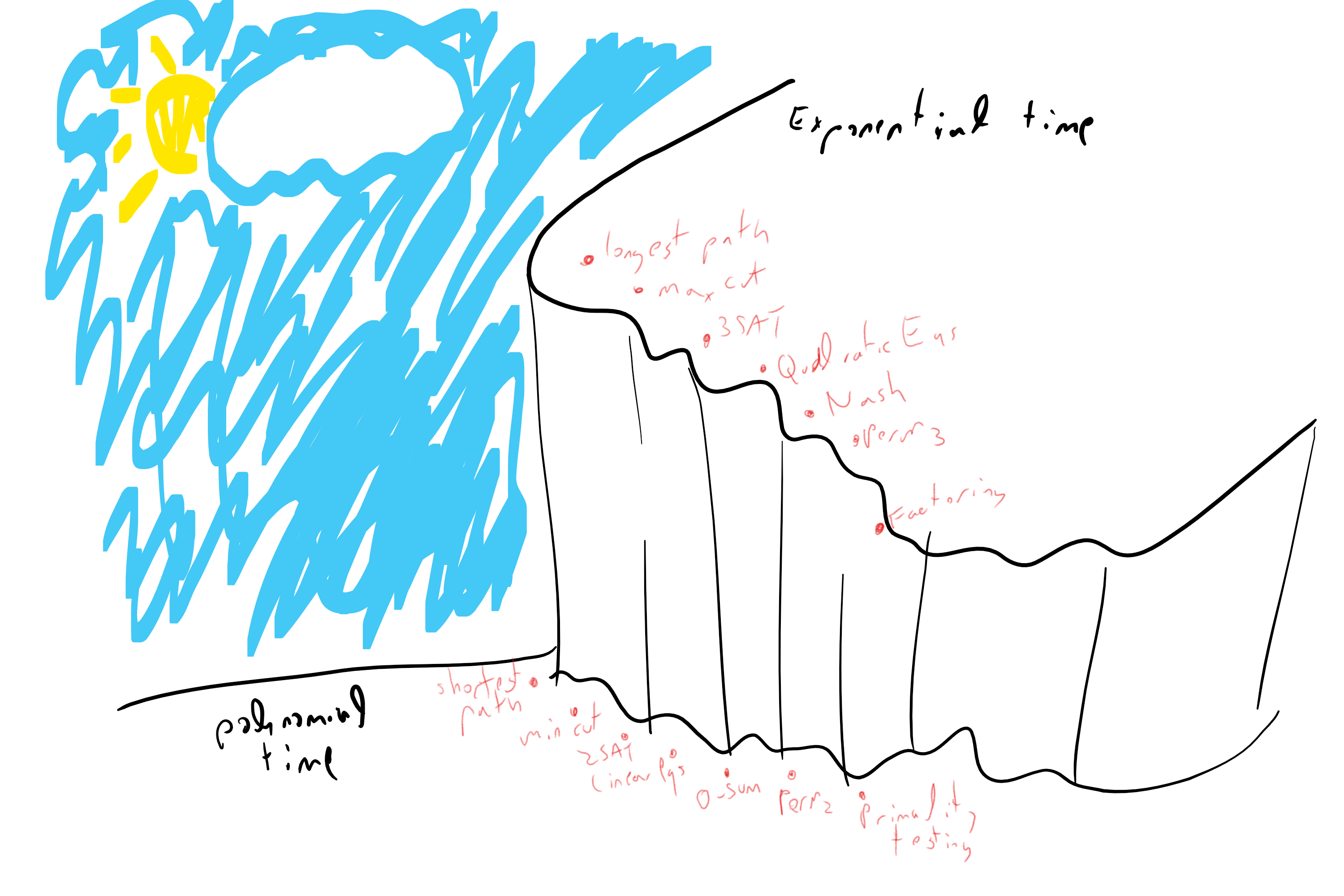
In this chapter, we informally survey examples of computational problems. For some of these problems we know efficient (i.e., \(O(n^c)\)-time for a small constant \(c\)) algorithms, and for others the best known algorithms are exponential.
We present these examples to get a feel as to the kinds of problems that lie on each side of this divide and also see how sometimes seemingly minor changes in problem formulation can make the (known) complexity of a problem “jump” from polynomial to exponential. We do not formally define the notion of running time in this chapter, but use the same “I know it when I see it” notion of an \(O(n)\) or \(O(n^2)\) time algorithms as the one you’ve seen in introduction to computer science courses. We will see the precise definition of running time (using Turing machines and RAM machines / NAND-RAM) in Chapter 13.
While the difference between \(O(n)\) and \(O(n^2)\) time can be crucial in practice, in this book we focus on the even bigger difference between polynomial and exponential running time. As we will see, the difference between polynomial versus exponential time is typically insensitive to the choice of the particular computational model, a polynomial-time algorithm is still polynomial whether you use Turing machines, RAM machines, or parallel cluster as your model of computation, and similarly an exponential-time algorithm will remain exponential in all of these platforms. One of the interesting phenomena of computing is that there is often a kind of a “threshold phenomenon” or “zero-one law” for running time. Many natural problems can either be solved in polynomial running time with a not-too-large exponent (e.g., something like \(O(n^2)\) or \(O(n^3)\)), or require exponential (e.g., at least \(2^{\Omega(n)}\) or \(2^{\Omega(\sqrt{n})}\)) time to solve. The reasons for this phenomenon are still not fully understood, but some light on it is shed by the concept of NP completeness, which we will see in Chapter 15.
This chapter is merely a tiny sample of the landscape of computational problems and efficient algorithms. If you want to explore the field of algorithms and data structures more deeply (which I very much hope you do!), the bibliographical notes contain references to some excellent texts, some of which are available freely on the web.
Part I of this book contained a quantitative study of computation of finite functions. We asked what are the resources (in terms of gates of Boolean circuits or lines in straight-line programs) required to compute various finite functions.
Part II of the book contained a qualitative study of computation of infinite functions (i.e., functions of unbounded input length). In that part we asked the qualitative question of whether or not a function is computable at all, regardless of the number of operations.
Part III of the book, beginning with this chapter, merges the two approaches and contains a quantitative study of computation of infinite functions. In this part we ask how do resources for computing a function scale with the length of the input. In Chapter 13 we define the notion of running time, and the class \(\mathbf{P}\) of functions that can be computed using a number of steps that scales polynomially with the input length. In Section 13.6 we will relate this class to the models of Boolean circuits and straightline programs that we studied in Part I.
Problems on graphs
In this chapter we discuss several examples of important computational problems. Many of the problems will involve graphs. We have already encountered graphs before (see Section 1.4.4) but now quickly recall the basic notation. A graph \(G\) consists of a set of vertices \(V\) and edges \(E\) where each edge is a pair of vertices. We typically denote by \(n\) the number of vertices (and in fact often consider graphs where the set of vertices \(V\) equals the set \([n]\) of the integers between \(0\) and \(n-1\)). In a directed graph, an edge is an ordered pair \((u,v)\), which we sometimes denote as \(\overrightarrow{u\;v}\). In an undirected graph, an edge is an unordered pair (or simply a set) \(\{ u,v \}\) which we sometimes denote as \(\overline{u\; v}\) or \(u \sim v\). An equivalent viewpoint is that an undirected graph corresponds to a directed graph satisfying the property that whenever the edge \(\overrightarrow{u\; v}\) is present then so is the edge \(\overrightarrow{v\; u}\). In this chapter we restrict our attention to graphs that are undirected and simple (i.e., containing no parallel edges or self-loops). Graphs can be represented either in the adjacency list or adjacency matrix representation. We can transform between these two representations using \(O(n^2)\) operations, and hence for our purposes we will mostly consider them as equivalent.
Graphs are so ubiquitous in computer science and other sciences because they can be used to model a great many of the data that we encounter. These are not just the “obvious” data such as the road network (which can be thought of as a graph of whose vertices are locations with edges corresponding to road segments), or the web (which can be thought of as a graph whose vertices are web pages with edges corresponding to links), or social networks (which can be thought of as a graph whose vertices are people and the edges correspond to friend relation). Graphs can also denote correlations in data (e.g., graph of observations of features with edges corresponding to features that tend to appear together), causal relations (e.g., gene regulatory networks, where a gene is connected to gene products it derives), or the state space of a system (e.g., graph of configurations of a physical system, with edges corresponding to states that can be reached from one another in one step).
Finding the shortest path in a graph
The shortest path problem is the task of finding, given a graph \(G=(V,E)\) and two vertices \(s,t \in V\), the length of the shortest path between \(s\) and \(t\) (if such a path exists). That is, we want to find the smallest number \(k\) such that there are vertices \(v_0,v_1,\ldots,v_k\) with \(v_0=s\), \(v_k=t\) and for every \(i\in\{0,\ldots,k-1\}\) an edge between \(v_i\) and \(v_{i+1}\). Formally, we define \(\ensuremath{\mathit{MINPATH}}:\{0,1\}^* \rightarrow \{0,1\}^*\) to be the function that on input a triple \((G,s,t)\) (represented as a string) outputs the number \(k\) which is the length of the shortest path in \(G\) between \(s\) and \(t\) or a string representing no path if no such path exists. (In practice people often want to also find the actual path and not just its length; it turns out that the algorithms to compute the length of the path often yield the actual path itself as a byproduct, and so everything we say about the task of computing the length also applies to the task of finding the path.)
If each vertex has at least two neighbors then there can be an exponential number of paths from \(s\) to \(t\), but fortunately we do not have to enumerate them all to find the shortest path. We can find the shortest path using a breadth first search (BFS), enumerating \(s\)’s neighbors, and then neighbors’ neighbors, etc.. in order. If we maintain the neighbors in a list we can perform a BFS in \(O(n^2)\) time, while using a queue we can do this in \(O(m)\) time, where \(m\) is the number of edges.1 Dijkstra’s algorithm is a well-known generalization of BFS to weighted graphs. More formally, the algorithm for computing the function \(\ensuremath{\mathit{MINPATH}}\) is described in Algorithm 12.2.
Algorithm 12.2 Shortest path via BFS
Input: Graph \(G=(V,E)\) and vertices \(s,t\in V\). Assume \(V=[n]\).
Output: Length \(k\) of shortest path from \(s\) to \(t\) or \(\infty\) if no such path exists.
Let \(D\) be length-\(n\) array.
Set \(D[s]=0\) and \(D[i]=\infty\) for all \(i\in [n] \setminus \{s \}\).
Initialize queue \(Q\) to contain \(s\).
while{\(Q\) non empty}
Pop \(v\) from \(Q\)
if{\(v=t\)}
return \(D[v]\)
endif
for{\(u\) neighbor of \(v\) with \(D[u]=\infty\)}
Set \(D[u] \leftarrow D[v]+1\)
Add \(u\) to \(Q\).
endfor
endwhile
return \(\infty\)
Since we only add to the queue vertices \(w\) with \(D[w]=\infty\) (and then immediately set \(D[w]\) to an actual number), we never push to the queue a vertex more than once, and hence the algorithm makes at most \(n\) “push” and “pop” operations. For each vertex \(v\), the number of times we run the inner loop is equal to the degree of \(v\) and hence the total running time is proportional to the sum of all degrees which equals twice the number \(m\) of edges. Algorithm 12.2 returns the correct answer since the vertices are added to the queue in the order of their distance from \(s\), and hence we will reach \(t\) after we have explored all the vertices that are closer to \(s\) than \(t\).
If you’ve ever taken an algorithms course, you have probably encountered many data structures such as lists, arrays, queues, stacks, heaps, search trees, hash tables and many more. Data structures are extremely important in computer science, and each one of those offers different tradeoffs between overhead in storage, operations supported, cost in time for each operation, and more. For example, if we store \(n\) items in a list, we will need a linear (i.e., \(O(n)\) time) scan to retrieve an element, while we achieve the same operation in \(O(1)\) time if we used a hash table. However, when we only care about polynomial-time algorithms, such factors of \(O(n)\) in the running time will not make much difference. Similarly, if we don’t care about the difference between \(O(n)\) and \(O(n^2)\), then it doesn’t matter if we represent graphs as adjacency lists or adjacency matrices. Hence we will often describe our algorithms at a very high level, without specifying the particular data structures that are used to implement them. However, it will always be clear that there exists some data structure that is sufficient for our purposes.
Finding the longest path in a graph
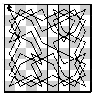
The longest path problem is the task of finding the length of the longest simple (i.e., non-intersecting) path between a given pair of vertices \(s\) and \(t\) in a given graph \(G\). If the graph is a road network, then the longest path might seem less motivated than the shortest path (unless you are the kind of person that always prefers the “scenic route”). But graphs can and are used to model a variety of phenomena, and in many such cases finding the longest path (and some of its variants) can be very useful. In particular, finding the longest path is a generalization of the famous Hamiltonian path problem which asks for a maximally long simple path (i.e., path that visits all \(n\) vertices once) between \(s\) and \(t\), as well as the notorious traveling salesman problem (TSP) of finding (in a weighted graph) a path visiting all vertices of cost at most \(w\). TSP is a classical optimization problem, with applications ranging from planning and logistics to DNA sequencing and astronomy.
Surprisingly, while we can find the shortest path in \(O(m)\) time, there is no known algorithm for the longest path problem that significantly improves on the trivial “exhaustive search” or “brute force” algorithm that enumerates all the exponentially many possibilities for such paths. Specifically, the best known algorithms for the longest path problem take \(O(c^n)\) time for some constant \(c>1\). (At the moment the best record is \(c \sim 1.65\) or so; even obtaining an \(O(2^n)\) time bound is not that simple, see Exercise 12.1.)
Finding the minimum cut in a graph
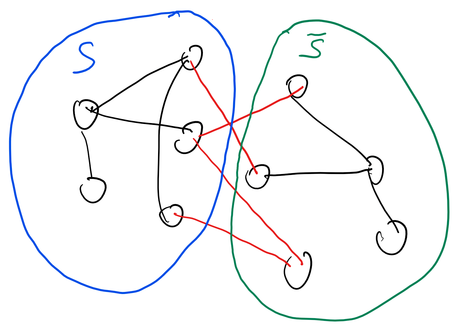
Given a graph \(G=(V,E)\), a cut of \(G\) is a subset \(S \subseteq V\) such that \(S\) is neither empty nor is it all of \(V\). The edges cut by \(S\) are those edges where one of their endpoints is in \(S\) and the other is in \(\overline{S} = V \setminus S\). We denote this set of edges by \(E(S,\overline{S})\). If \(s,t \in V\) are a pair of vertices then an \(s,t\) cut is a cut such that \(s\in S\) and \(t\in \overline{S}\) (see Figure 12.3). The minimum \(s,t\) cut problem is the task of finding, given \(s\) and \(t\), the minimum number \(k\) such that there is an \(s,t\) cut cutting \(k\) edges (the problem is also sometimes phrased as finding the set that achieves this minimum; it turns out that algorithms to compute the number often yield the set as well). Formally, we define \(\ensuremath{\mathit{MINCUT}}:\{0,1\}^* \rightarrow \{0,1\}^*\) to be the function that on input a string representing a triple \((G=(V,E),s,t)\) of a graph and two vertices, outputs the minimum number \(k\) such that there exists a set \(S \subseteq V\) with \(s\in S\), \(t\not\in S\) and \(|E(S,\overline{S})|=k\).
Computing minimum \(s,t\) cuts is useful in many applications since minimum cuts often correspond to bottlenecks. For example, in a communication or railroad network the minimum cut between \(s\) and \(t\) corresponds to the smallest number of edges that, if dropped, will disconnect \(s\) from \(t\). (This was actually the original motivation for this problem; see Section 12.6.) Similar applications arise in scheduling and planning. In the setting of image segmentation, one can define a graph whose vertices are pixels and whose edges correspond to neighboring pixels of distinct colors. If we want to separate the foreground from the background then we can pick (or guess) a foreground pixel \(s\) and background pixel \(t\) and ask for a minimum cut between them.
The naive algorithm for computing \(\ensuremath{\mathit{MINCUT}}\) will check all \(2^n\) possible subsets of an \(n\)-vertex graph, but it turns out we can do much better than that. As we’ve seen in this book time and again, there is more than one algorithm to compute the same function, and some of those algorithms might be more efficient than others. Luckily the minimum cut problem is one of those cases. In particular, as we will see in the next section, there are algorithms that compute \(\ensuremath{\mathit{MINCUT}}\) in time which is polynomial in the number of vertices.
Min-Cut Max-Flow and Linear programming
We can obtain a polynomial-time algorithm for computing \(\ensuremath{\mathit{MINCUT}}\) using the Max-Flow Min-Cut Theorem. This theorem says that the minimum cut between \(s\) and \(t\) equals the maximum amount of flow we can send from \(s\) to \(t\), if every edge has unit capacity. Specifically, imagine that every edge of the graph corresponded to a pipe that could carry one unit of fluid per one unit of time (say 1 liter of water per second). The maximum \(s,t\) flow is the maximum units of water that we could transfer from \(s\) to \(t\) over these pipes. If there is an \(s,t\) cut of \(k\) edges, then the maximum flow is at most \(k\). The reason is that such a cut \(S\) acts as a “bottleneck” since at most \(k\) units can flow from \(S\) to its complement at any given unit of time. This means that the maximum \(s,t\) flow is always at most the value of the minimum \(s,t\) cut. The surprising and non-trivial content of the Max-Flow Min-Cut Theorem is that the maximum flow is also at least the value of the minimum cut, and hence computing the cut is the same as computing the flow.
The Max-Flow Min-Cut Theorem reduces the task of computing a minimum cut to the task of computing a maximum flow. However, this still does not show how to compute such a flow. The Ford-Fulkerson Algorithm is a direct way to compute a flow using incremental improvements. But computing flows in polynomial time is also a special case of a much more general tool known as linear programming.
A flow on a graph \(G\) of \(m\) edges can be modeled as a vector \(x\in \R^m\) where for every edge \(e\), \(x_e\) corresponds to the amount of water per time-unit that flows on \(e\). We think of an edge \(e\) as an ordered pair \((u,v)\) (we can choose the order arbitrarily) and let \(x_e\) be the amount of flow that goes from \(u\) to \(v\). (If the flow is in the other direction then we make \(x_e\) negative.) Since every edge has capacity one, we know that \(-1 \leq x_e \leq 1\) for every edge \(e\). A valid flow has the property that the amount of water leaving the source \(s\) is the same as the amount entering the sink \(t\), and that for every other vertex \(v\), the amount of water entering and leaving \(v\) is the same.
Mathematically, we can write these conditions as follows:
where for every vertex \(v\), summing over \(e \ni v\) means summing over all the edges that touch \(v\).
The maximum flow problem can be thought of as the task of maximizing \(\sum_{e \ni s} x_e\) over all the vectors \(x\in\R^m\) that satisfy the above conditions Equation 12.1. Maximizing a linear function \(\ell(x)\) over the set of \(x\in \R^m\) that satisfy certain linear equalities and inequalities is known as linear programming. Luckily, there are polynomial-time algorithms for solving linear programming, and hence we can solve the maximum flow (and so, equivalently, minimum cut) problem in polynomial time. In fact, there are much better algorithms for maximum-flow/minimum-cut, even for weighted directed graphs, with currently the record standing at \(O(\min\{ m^{10/7}, m\sqrt{n}\})\) time.
Given a graph \(G=(V,E)\), define the global minimum cut of \(G\) to be the minimum over all \(S \subseteq V\) with \(S \neq \emptyset\) and \(S \neq V\) of the number of edges cut by \(S\). Prove that there is a polynomial-time algorithm to compute the global minimum cut of a graph.
By the above we know that there is a polynomial-time algorithm \(A\) that on input \((G,s,t)\) finds the minimum \(s,t\) cut in the graph \(G\). Using \(A\), we can obtain an algorithm \(B\) that on input a graph \(G\) computes the global minimum cut as follows:
For every distinct pair \(s,t \in V\), Algorithms \(B\) sets \(k_{s,t}\leftarrow A(G,s,t)\).
\(B\) returns the minimum of \(k_{s,t}\) over all distinct pairs \(s,t\)
The running time of \(B\) will be \(O(n^2)\) times the running time of \(A\) and hence polynomial time. Moreover, if the global minimum cut is \(S\), then when \(B\) reaches an iteration with \(s\in S\) and \(t\not\in S\) it will obtain the value of this cut, and hence the value output by \(B\) will be the value of the global minimum cut.
The above is our first example of a reduction in the context of polynomial-time algorithms. Namely, we reduced the task of computing the global minimum cut to the task of computing minimum \(s,t\) cuts.
Finding the maximum cut in a graph
The maximum cut problem is the task of finding, given an input graph \(G=(V,E)\), the subset \(S\subseteq V\) that maximizes the number of edges cut by \(S\). (We can also define an \(s,t\)-cut variant of the maximum cut like we did for minimum cut; the two variants have similar complexity but the global maximum cut is more common in the literature.) Like its cousin the minimum cut problem, the maximum cut problem is also very well motivated. For example, maximum cut arises in VLSI design, and also has some surprising relation to analyzing the Ising model in statistical physics.
Surprisingly, while (as we’ve seen) there is a polynomial-time algorithm for the minimum cut problem, there is no known algorithm solving maximum cut much faster than the trivial “brute force” algorithm that tries all \(2^n\) possibilities for the set \(S\).
A note on convexity
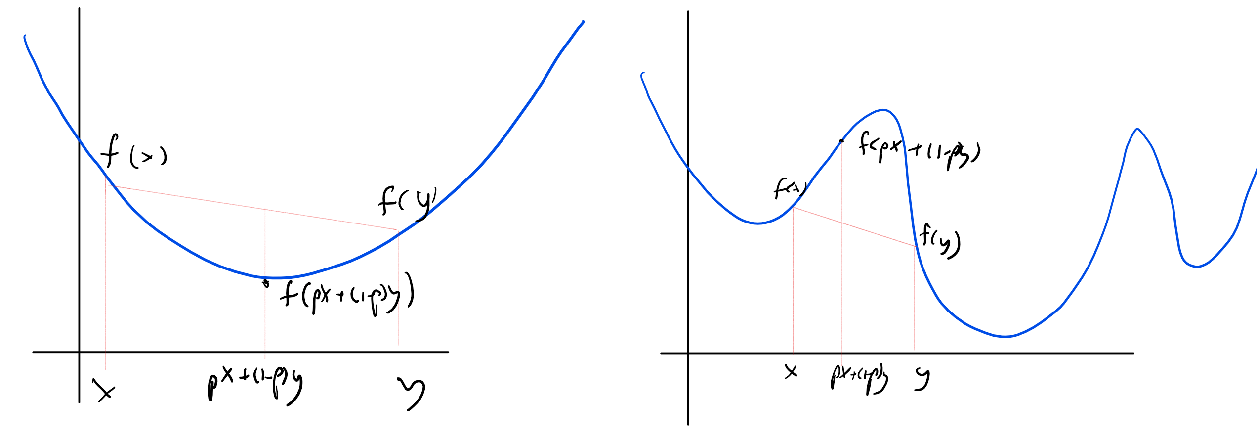
There is an underlying reason for the sometimes radical difference between the difficulty of maximizing and minimizing a function over a domain. If \(D \subseteq \R^n\), then a function \(f:D \rightarrow R\) is convex if for every \(x,y \in D\) and \(p\in [0,1]\) \(f(px+(1-p)y) \leq pf(x) + (1-p)f(y)\). That is, \(f\) applied to the \(p\)-weighted midpoint between \(x\) and \(y\) is smaller than the \(p\)-weighted average value of \(f\). If \(D\) itself is convex (which means that if \(x,y\) are in \(D\) then so is the line segment between them), then this means that if \(x\) is a local minimum of \(f\) then it is also a global minimum. The reason is that if \(f(y)<f(x)\) then every point \(z=px+(1-p)y\) on the line segment between \(x\) and \(y\) will satisfy \(f(z) \leq p f(x) + (1-p)f(y) < f(x)\) and hence in particular \(x\) cannot be a local minimum. Intuitively, local minima of functions are much easier to find than global ones: after all, any “local search” algorithm that keeps finding a nearby point on which the value is lower, will eventually arrive at a local minimum. One example of such a local search algorithm is gradient descent which takes a sequence of small steps, each one in the direction that would reduce the value by the most amount based on the current derivative.
Indeed, under certain technical conditions, we can often efficiently find the minimum of convex functions over a convex domain, and this is the reason why problems such as minimum cut and shortest path are easy to solve. On the other hand, maximizing a convex function over a convex domain (or equivalently, minimizing a concave function) can often be a hard computational task. A linear function is both convex and concave, which is the reason that both the maximization and minimization problems for linear functions can be done efficiently.
The minimum cut problem is not a priori a convex minimization task, because the set of potential cuts is discrete and not continuous. However, it turns out that we can embed it in a continuous and convex set via the (linear) maximum flow problem. The “max flow min cut” theorem ensures that this embedding is “tight” in the sense that the minimum “fractional cut” that we obtain through the maximum-flow linear program will be the same as the true minimum cut. Unfortunately, we don’t know of such a tight embedding in the setting of the maximum cut problem.
Convexity arises time and again in the context of efficient computation. For example, one of the basic tasks in machine learning is empirical risk minimization. This is the task of finding a classifier for a given set of training examples. That is, the input is a list of labeled examples \((x_0,y_0),\ldots,(x_{m-1},y_{m-1})\), where each \(x_i \in \{0,1\}^n\) and \(y_i \in \{0,1\}\), and the goal is to find a classifier \(h:\{0,1\}^n \rightarrow \{0,1\}\) (or sometimes \(h:\{0,1\}^n \rightarrow \R\)) that minimizes the number of errors. More generally, we want to find \(h\) that minimizes
Beyond graphs
Not all computational problems arise from graphs. We now list some other examples of computational problems that are of great interest.
SAT
A propositional formula \(\varphi\) involves \(n\) variables \(x_1,\ldots,x_n\) and the logical operators AND (\(\wedge\)), OR (\(\vee\)), and NOT (\(\neg\), also denoted as \(\overline{\cdot}\)). We say that such a formula is in conjunctive normal form (CNF for short) if it is an AND of ORs of variables or their negations (we call a term of the form \(x_i\) or \(\overline{x}_i\) a literal). For example, this is a CNF formula
The satisfiability problem is the task of determining, given a CNF formula \(\varphi\), whether or not there exists a satisfying assignment for \(\varphi\). A satisfying assignment for \(\varphi\) is a string \(x\in \{0,1\}^n\) such that \(\varphi\) evaluates to True if we assign its variables the values of \(x\). The SAT problem might seem as an abstract question of interest only in logic but in fact SAT is of huge interest in industrial optimization, with applications including manufacturing planning, circuit synthesis, software verification, air-traffic control, scheduling sports tournaments, and more.
2SAT. We say that a formula is a \(k\)-CNF it is an AND of ORs where each OR involves exactly \(k\) literals. The \(k\)-SAT problem is the restriction of the satisfiability problem for the case that the input formula is a \(k\)-CNF. In particular, the 2SAT problem is to find out, given a \(2\)-CNF formula \(\varphi\), whether there is an assignment \(x\in \{0,1\}^n\) that satisfies \(\varphi\), in the sense that it makes it evaluate to \(1\) or “True”. The trivial, brute-force, algorithm for 2SAT will enumerate all the \(2^n\) assignments \(x\in \{0,1\}^n\) but fortunately we can do much better. The key is that we can think of every constraint of the form \(\ell_i \vee \ell_j\) (where \(\ell_i,\ell_j\) are literals, corresponding to variables or their negations) as an implication \(\overline{\ell}_i \Rightarrow \ell_j\), since it corresponds to the constraints that if the literal \(\ell'_i = \overline{\ell}_i\) is true then it must be the case that \(\ell_j\) is true as well. Hence we can think of \(\varphi\) as a directed graph between the \(2n\) literals, with an edge from \(\ell_i\) to \(\ell_j\) corresponding to an implication from the former to the latter. It can be shown that \(\varphi\) is unsatisfiable if and only if there is a variable \(x_i\) such that there is a directed path from \(x_i\) to \(\overline{x}_i\) as well as a directed path from \(\overline{x}_i\) to \(x_i\) (see Exercise 12.2). This reduces 2SAT to the (efficiently solvable) problem of determining connectivity in directed graphs.
3SAT. The 3SAT problem is the task of determining satisfiability for 3CNFs. One might think that changing from two to three would not make that much of a difference for complexity. One would be wrong. Despite much effort, we do not know of a significantly better than brute force algorithm for 3SAT (the best known algorithms take roughly \(1.3^n\) steps).
Interestingly, a similar issue arises time and again in computation, where the difference between two and three often corresponds to the difference between tractable and intractable. We do not fully understand the reasons for this phenomenon, though the notion of \(\mathbf{NP}\) completeness we will see later does offer a partial explanation. It may be related to the fact that optimizing a polynomial often amounts to equations on its derivative. The derivative of a quadratic polynomial is linear, while the derivative of a cubic is quadratic, and, as we will see, the difference between solving linear and quadratic equations can be quite profound.
Solving linear equations
One of the most useful problems that people have been solving time and again is solving \(n\) linear equations in \(n\) variables. That is, solve equations of the form
where \(\{ a_{i,j} \}_{i,j \in [n]}\) and \(\{ b_i \}_{i\in [n]}\) are real (or rational) numbers. More compactly, we can write this as the equations \(Ax = b\) where \(A\) is an \(n\times n\) matrix, and we think of \(x,b\) are column vectors in \(\R^n\).
The standard Gaussian elimination algorithm can be used to solve such equations in polynomial time (i.e., determine if they have a solution, and if so, to find it). As we discussed above, if we are willing to allow some loss in precision, we even have algorithms that handle linear inequalities, also known as linear programming. In contrast, if we insist on integer solutions, the task of solving for linear equalities or inequalities is known as integer programming, and the best known algorithms are exponential time in the worst case.
Whenever we discuss problems whose inputs correspond to numbers, the input length corresponds to how many bits are needed to describe the number (or, as is equivalent up to a constant factor, the number of digits in base 10, 16 or any other constant). The difference between the length of the input and the magnitude of the number itself can be of course quite profound. For example, most people would agree that there is a huge difference between having a billion (i.e. \(10^9\)) dollars and having nine dollars. Similarly there is a huge difference between an algorithm that takes \(n\) steps on an \(n\)-bit number and an algorithm that takes \(2^n\) steps.
One example is the problem (discussed below) of finding the prime factors of a given integer \(N\). The natural algorithm is to search for such a factor by trying all numbers from \(1\) to \(N\), but that would take \(N\) steps which is exponential in the input length, which is the number of bits needed to describe \(N\). (The running time of this algorithm can be easily improved to roughly \(\sqrt{N}\), but this is still exponential (i.e., \(2^{n/2}\)) in the number \(n\) of bits to describe \(N\).) It is an important and long open question whether there is such an algorithm that runs in time polynomial in the input length (i.e., polynomial in \(\log N\)).
Solving quadratic equations
Suppose that we want to solve not just linear but also equations involving quadratic terms of the form \(a_{i,j,k}x_jx_k\). That is, suppose that we are given a set of quadratic polynomials \(p_1,\ldots,p_m\) and consider the equations \(\{ p_i(x) = 0 \}\). To avoid issues with bit representations, we will always assume that the equations contain the constraints \(\{ x_i^2 - x_i = 0 \}_{i\in [n]}\). Since only \(0\) and \(1\) satisfy the equation \(a^2-a=0\), this assumption means that we can restrict attention to solutions in \(\{0,1\}^n\). Solving quadratic equations in several variables is a classical and extremely well motivated problem. This is the generalization of the classical case of single-variable quadratic equations that generations of high school students grapple with. It also generalizes the quadratic assignment problem, introduced in the 1950’s as a way to optimize assignment of economic activities. Once again, we do not know a much better algorithm for this problem than the one that enumerates over all the \(2^n\) possibilities.
More advanced examples
We now list a few more examples of interesting problems that are a little more advanced but are of significant interest in areas such as physics, economics, number theory, and cryptography.
Determinant of a matrix
The determinant of a \(n\times n\) matrix \(A\), denoted by \(\mathrm{det}(A)\), is an extremely important quantity in linear algebra. For example, it is known that \(\mathrm{det}(A) \neq 0\) if and only if \(A\) is non-singular, which means that it has an inverse \(A^{-1}\), and hence we can always uniquely solve equations of the form \(Ax = b\) where \(x\) and \(b\) are \(n\)-dimensional vectors. More generally, the determinant can be thought of as a quantitative measure as to what extent \(A\) is far from being singular. If the rows of \(A\) are “almost” linearly dependent (for example, if the third row is very close to being a linear combination of the first two rows) then the determinant will be small, while if they are far from it (for example, if they are are orthogonal to one another, then the determinant will be large). In particular, for every matrix \(A\), the absolute value of the determinant of \(A\) is at most the product of the norms (i.e., square root of sum of squares of entries) of the rows, with equality if and only if the rows are orthogonal to one another.
The determinant can be defined in several ways. One way to define the determinant of an \(n\times n\) matrix \(A\) is:
where \(S_n\) is the set of all permutations from \([n]\) to \([n]\) and the sign of a permutation \(\pi\) is equal to \(-1\) raised to the power of the number of inversions in \(\pi\) (pairs \(i,j\) such that \(i>j\) but \(\pi(i)<\pi(j)\)).
This definition suggests that computing \(\mathrm{det}(A)\) might require summing over \(|S_n|\) terms which would take exponential time since \(|S_n| = n! > 2^n\). However, there are other ways to compute the determinant. For example, it is known that \(\mathrm{det}\) is the only function that satisfies the following conditions:
\(\mathrm{det}(\ensuremath{\mathit{AB}}) = \mathrm{det}(A)\mathrm{det}(B)\) for every square matrices \(A,B\).
For every \(n\times n\) triangular matrix \(T\) with diagonal entries \(d_0,\ldots, d_{n-1}\), \(\mathrm{det}(T)=\prod_{i=0}^n d_i\). In particular \(\mathrm{det}(I)=1\) where \(I\) is the identity matrix. (A triangular matrix is one in which either all entries below the diagonal, or all entries above the diagonal, are zero.)
\(\mathrm{det}(S)=-1\) where \(S\) is a “swap matrix” that corresponds to swapping two rows or two columns of \(I\). That is, there are two coordinates \(a,b\) such that for every \(i,j\), \(S_{i,j} = \begin{cases}1 & i=j\;, i \not\in \{a,b \} \\ 1 & \{i,j\}=\{a,b\} \\ 0 & \text{otherwise}\end{cases}\).
Using these rules and the Gaussian elimination algorithm, it is possible to tell whether \(A\) is singular or not, and in the latter case, decompose \(A\) as a product of a polynomial number of swap matrices and triangular matrices. (Indeed one can verify that the row operations in Gaussian elimination corresponds to either multiplying by a swap matrix or by a triangular matrix.) Hence we can compute the determinant for an \(n\times n\) matrix using a polynomial time of arithmetic operations.
Permanent of a matrix
Given an \(n\times n\) matrix \(A\), the permanent of \(A\) is defined as
That is, \(\mathrm{perm}(A)\) is defined analogously to the determinant in Equation 12.2 except that we drop the term \(\mathrm{sign}(\pi)\). The permanent of a matrix is a natural quantity, and has been studied in several contexts including combinatorics and graph theory. It also arises in physics where it can be used to describe the quantum state of multiple Boson particles (see here and here).
Permanent modulo 2. If the entries of \(A\) are integers, then we can define the Boolean function \(perm_2\) which outputs on input a matrix \(A\) the result of the permanent of \(A\) modulo \(2\). It turns out that we can compute \(perm_2(A)\) in polynomial time. The key is that modulo \(2\), \(-x\) and \(+x\) are the same quantity and hence, since the only difference between Equation 12.2 and Equation 12.3 is that some terms are multiplied by \(-1\), \(\mathrm{det}(A) \mod 2 = \mathrm{perm}(A) \mod 2\) for every \(A\).
Permanent modulo 3. Emboldened by our good fortune above, we might hope to be able to compute the permanent modulo any prime \(p\) and perhaps in full generality. Alas, we have no such luck. In a similar “two to three” type of a phenomenon, we do not know of a much better than brute force algorithm to even compute the permanent modulo \(3\).
Finding a zero-sum equilibrium
A zero sum game is a game between two players where the payoff for one is the same as the penalty for the other. That is, whatever the first player gains, the second player loses. As much as we want to avoid them, zero sum games do arise in life, and the one good thing about them is that at least we can compute the optimal strategy.
A zero sum game can be specified by an \(n\times n\) matrix \(A\), where if player 1 chooses action \(i\) and player 2 chooses action \(j\) then player one gets \(A_{i,j}\) and player 2 loses the same amount. The famous Min Max Theorem by John von Neumann states that if we allow probabilistic or “mixed” strategies (where a player does not choose a single action but rather a distribution over actions) then it does not matter who plays first: the end result will be the same. Mathematically the min max theorem is that if we let \(\Delta_n\) be the set of probability distributions over \([n]\) (i.e., non-negative columns vectors in \(\R^n\) whose entries sum to \(1\)) then
The min-max theorem turns out to be a corollary of linear programming duality, and indeed the value of Equation 12.4 can be computed efficiently by a linear program.
Finding a Nash equilibrium
Fortunately, not all real-world games are zero sum, and we do have more general games, where the payoff of one player does not necessarily equal the loss of the other. John Nash won the Nobel prize for showing that there is a notion of equilibrium for such games as well. In many economic texts it is taken as an article of faith that when actual agents are involved in such a game then they reach a Nash equilibrium. However, unlike zero sum games, we do not know of an efficient algorithm for finding a Nash equilibrium given the description of a general (non-zero-sum) game. In particular this means that, despite economists’ intuitions, there are games for which natural strategies will take an exponential number of steps to converge to an equilibrium.
Primality testing
Another classical computational problem, that has been of interest since the ancient Greeks, is to determine whether a given number \(N\) is prime or composite. Clearly we can do so by trying to divide it with all the numbers in \(2,\ldots,N-1\), but this would take at least \(N\) steps which is exponential in its bit complexity \(n = \log N\). We can reduce these \(N\) steps to \(\sqrt{N}\) by observing that if \(N\) is a composite of the form \(N=\ensuremath{\mathit{PQ}}\) then either \(P\) or \(Q\) is smaller than \(\sqrt{N}\). But this is still quite terrible. If \(N\) is a \(1024\) bit integer, \(\sqrt{N}\) is about \(2^{512}\), and so running this algorithm on such an input would take much more than the lifetime of the universe.
Luckily, it turns out we can do radically better. In the 1970’s, Rabin and Miller gave probabilistic algorithms to determine whether a given number \(N\) is prime or composite in time \(poly(n)\) for \(n=\log N\). We will discuss the probabilistic model of computation later in this course. In 2002, Agrawal, Kayal, and Saxena found a deterministic \(poly(n)\) time algorithm for this problem. This is surely a development that mathematicians from Archimedes till Gauss would have found exciting.
Integer factoring
Given that we can efficiently determine whether a number \(N\) is prime or composite, we could expect that in the latter case we could also efficiently find the factorization of \(N\). Alas, no such algorithm is known. In a surprising and exciting turn of events, the non-existence of such an algorithm has been used as a basis for encryptions, and indeed it underlies much of the security of the world wide web. We will return to the factoring problem later in this course. We remark that we do know much better than brute force algorithms for this problem. While the brute force algorithms would require \(2^{\Omega(n)}\) time to factor an \(n\)-bit integer, there are known algorithms running in time roughly \(2^{O(\sqrt{n})}\) and also algorithms that are widely believed (though not fully rigorously analyzed) to run in time roughly \(2^{O(n^{1/3})}\). (By “roughly” we mean that we neglect factors that are polylogarithmic in \(n\).)
Our current knowledge
The difference between an exponential and polynomial time algorithm might seem merely “quantitative” but it is in fact extremely significant. As we’ve already seen, the brute force exponential time algorithm runs out of steam very very fast, and as Edmonds says, in practice there might not be much difference between a problem where the best algorithm is exponential and a problem that is not solvable at all. Thus the efficient algorithms we mentioned above are widely used and power many computer science applications. Moreover, a polynomial-time algorithm often arises out of significant insight to the problem at hand, whether it is the “max-flow min-cut” result, the solvability of the determinant, or the group theoretic structure that enables primality testing. Such insight can be useful regardless of its computational implications.
At the moment we do not know whether the “hard” problems are truly hard, or whether it is merely because we haven’t yet found the right algorithms for them. However, we will now see that there are problems that do inherently require exponential time. We just don’t know if any of the examples above fall into that category.
There are many natural problems that have polynomial-time algorithms, and other natural problems that we’d love to solve, but for which the best known algorithms are exponential.
Often a polynomial time algorithm relies on discovering some hidden structure in the problem, or finding a surprising equivalent formulation for it.
There are many interesting problems where there is an exponential gap between the best known algorithm and the best algorithm that we can rule out. Closing this gap is one of the main open questions of theoretical computer science.
Exercises
The naive algorithm for computing the longest path in a given graph could take more than \(n!\) steps. Give a \(poly(n)2^n\) time algorithm for the longest path problem in \(n\) vertex graphs.2
For every 2CNF \(\varphi\), define the graph \(G_\varphi\) on \(2n\) vertices corresponding to the literals \(x_1,\ldots,x_n,\overline{x}_1,\ldots,\overline{x}_n\), such that there is an edge \(\overrightarrow{\ell_i\; \ell_j}\) iff the constraint \(\overline{\ell}_i \vee \ell_j\) is in \(\varphi\). Prove that \(\varphi\) is unsatisfiable if and only if there is some \(i\) such that there is a path from \(x_i\) to \(\overline{x}_i\) and from \(\overline{x}_i\) to \(x_i\) in \(G_\varphi\). Show how to use this to solve 2SAT in polynomial time.
The following fact is true: there is a polynomial-time algorithm \(\ensuremath{\mathit{BIP}}\) that on input a graph \(G=(V,E)\) outputs \(1\) if and only if the graph is bipartite: there is a partition of \(V\) to disjoint parts \(S\) and \(T\) such that every edge \((u,v) \in E\) satisfies either \(u\in S\) and \(v\in T\) or \(u\in T\) and \(v\in S\). Use this fact to prove that there is a polynomial-time algorithm to compute that following function \(\ensuremath{\mathit{CLIQUEPARTITION}}\) that on input a graph \(G=(V,E)\) outputs \(1\) if and only if there is a partition of \(V\) the graph into two parts \(S\) and \(T\) such that both \(S\) and \(T\) are cliques: for every pair of distinct vertices \(u,v \in S\), the edge \((u,v)\) is in \(E\) and similarly for every pair of distinct vertices \(u,v \in T\), the edge \((u,v)\) is in \(E\).
Bibliographical notes
The classic undergraduate introduction to algorithms text is (Cormen, Leiserson, Rivest, Stein, 2009) . Two texts that are less “encyclopedic” are Kleinberg and Tardos (Kleinberg, Tardos, 2006) , and Dasgupta, Papadimitriou and Vazirani (Dasgupta, Papadimitriou, Vazirani, 2008) . Jeff Erickson’s book is an excellent algorithms text that is freely available online.
The origins of the minimum cut problem date to the Cold War. Specifically, Ford and Fulkerson discovered their max-flow/min-cut algorithm in 1955 as a way to find out the minimum amount of train tracks that would need to be blown up to disconnect Russia from the rest of Europe. See the survey (Schrijver, 2005) for more.
Some algorithms for the longest path problem are given in (Williams, 2009) (Bjorklund, 2014) .
Further explorations
Some topics related to this chapter that might be accessible to advanced students include: (to be completed)
- ↩
A queue is a data structure for storing a list of elements in “First In First Out (FIFO)” order. Each “pop” operation removes an element from the queue in the order that they were “pushed” into it; see the Wikipedia page.
- ↩
Hint: Use dynamic programming to compute for every \(s,t \in [n]\) and \(S \subseteq [n]\) the value \(P(s,t,S)\) which equals \(1\) if there is a simple path from \(s\) to \(t\) that uses exactly the vertices in \(S\). Do this iteratively for \(S\)’s of growing sizes.
Comments
Comments are posted on the GitHub repository using the utteranc.es app. A GitHub login is required to comment. If you don't want to authorize the app to post on your behalf, you can also comment directly on the GitHub issue for this page.
Compiled on 12/06/2023 00:06:51
Copyright 2023, Boaz Barak.

This work is
licensed under a Creative Commons
Attribution-NonCommercial-NoDerivatives 4.0 International License.
Produced using pandoc and panflute with templates derived from gitbook and bookdown.