See any bugs/typos/confusing explanations? Open a GitHub issue. You can also comment below
★ See also the PDF version of this chapter (better formatting/references) ★
Is every theorem provable?
- More examples of uncomputable functions that are not as tied to computation.
- Gödel’s incompleteness theorem - a result that shook the world of mathematics in the early 20th century.
“Take any definite unsolved problem, such as … the existence of an infinite number of prime numbers of the form \(2^n + 1\). However unapproachable these problems may seem to us and however helpless we stand before them, we have, nevertheless, the firm conviction that their solution must follow by a finite number of purely logical processes…”
“…This conviction of the solvability of every mathematical problem is a powerful incentive to the worker. We hear within us the perpetual call: There is the problem. Seek its solution. You can find it by pure reason, for in mathematics there is no ignorabimus.”, David Hilbert, 1900.
“The meaning of a statement is its method of verification.”, Moritz Schlick, 1938 (aka “The verification principle” of logical positivism)
The problems shown uncomputable in Chapter 9, while natural and important, still intimately involved NAND-TM programs or other computing mechanisms in their definitions. One could perhaps hope that as long as we steer clear of functions whose inputs are themselves programs, we can avoid the “curse of uncomputability”. Alas, we have no such luck.
In this chapter we will see an example of a natural and seemingly “computation free” problem that nevertheless turns out to be uncomputable: solving Diophantine equations. As a corollary, we will see one of the most striking results of 20th century mathematics: Gödel’s Incompleteness Theorem, which showed that there are some mathematical statements (in fact, in number theory) that are inherently unprovable. We will actually start with the latter result, and then show the former.
The marquee result of this chapter is Gödel’s Incompleteness Theorem, which states that for every proof system, there are some statements about arithmetic that are true but unprovable in this system. But more than that we will see a deep connection between uncomputability and unprovability. For example, the uncomputability of the Halting problem immediately gives rise to the existence of unprovable statements about Turing machines. To even state Gödel’s Incompleteness Theorem we will need to formally define the notion of a “proof system”. We give a very general definition, that encompasses all types of “axioms + inference rules” systems used in logic and math. We will then build up the machinery to encode computation using arithmetic that will enable us to prove Gödel’s Theorem.
Hilbert’s Program and Gödel’s Incompleteness Theorem
“And what are these …vanishing increments? They are neither finite quantities, nor quantities infinitely small, nor yet nothing. May we not call them the ghosts of departed quantities?”, George Berkeley, Bishop of Cloyne, 1734.
The 1700’s and 1800’s were a time of great discoveries in mathematics but also of several crises. The discovery of calculus by Newton and Leibnitz in the late 1600’s ushered a golden age of problem solving. Many longstanding challenges succumbed to the new tools that were discovered, and mathematicians got ever better at doing some truly impressive calculations. However, the rigorous foundations behind these calculations left much to be desired. Mathematicians manipulated infinitesimal quantities and infinite series cavalierly, and while most of the time they ended up with the correct results, there were a few strange examples (such as trying to calculate the value of the infinite series \(1-1+1-1+1+\ldots\)) which seemed to give out different answers depending on the method of calculation. This led to a growing sense of unease in the foundations of the subject which was addressed in the works of mathematicians such as Cauchy, Weierstrass, and Riemann, who eventually placed analysis on firmer foundations, giving rise to the \(\epsilon\)’s and \(\delta\)’s that students taking honors calculus grapple with to this day.
In the beginning of the 20th century, there was an effort to replicate this effort, in greater rigor, to all parts of mathematics. The hope was to show that all the true results of mathematics can be obtained by starting with a number of axioms, and deriving theorems from them using logical rules of inference. This effort was known as the Hilbert program, named after the influential mathematician David Hilbert.
Alas, it turns out the results we’ve seen dealt a devastating blow to this program, as was shown by Kurt Gödel in 1931:
For every sound proof system \(V\) for sufficiently rich mathematical statements, there is a mathematical statement that is true but is not provable in \(V\).
Defining “Proof Systems”
Before proving Theorem 11.1, we need to define “proof systems” and even formally define the notion of a “mathematical statement”. In geometry and other areas of mathematics, proof systems are often defined by starting with some basic assumptions or axioms and then deriving more statements by using inference rules such as the famous Modus Ponens, but what axioms shall we use? What rules? We will use an extremely general notion of proof systems, not even restricting ourselves to ones that have the form of axioms and inference.
Mathematical statements. At the highest level, a mathematical statement is simply a piece of text, which we can think of as a string \(x\in \{0,1\}^*\). Mathematical statements contain assertions whose truth does not depend on any empirical fact, but rather only on properties of abstract objects. For example, the following is a mathematical statement:1
“The number \(2\),\(696\),\(635\),\(869\),\(504\),\(783\),\(333\),\(238\),\(805\),\(675\),\(613\), \(588\),\(278\),\(597\),\(832\),\(162\),\(617\),\(892\),\(474\),\(670\),\(798\),\(113\) is prime”.
Mathematical statements do not have to involve numbers. They can assert properties of any other mathematical object including sets, strings, functions, graphs and yes, even programs. Thus, another example of a mathematical statement is the following:2
Proof systems. A proof for a statement \(x\in \{0,1\}^*\) is another piece of text \(w\in \{0,1\}^*\) that certifies the truth of the statement asserted in \(x\). The conditions for a valid proof system are:
(Effectiveness) Given a statement \(x\) and a proof \(w\), there is an algorithm to verify whether or not \(w\) is a valid proof for \(x\). (For example, by going line by line and checking that each line follows from the preceding ones using one of the allowed inference rules.)
(Soundness) If there is a valid proof \(w\) for \(x\) then \(x\) is true.
These are quite minimal requirements for a proof system. Requirement 2 (soundness) is the very definition of a proof system: you shouldn’t be able to prove things that are not true. Requirement 1 is also essential. If there is no set of rules (i.e., an algorithm) to check that a proof is valid then in what sense is it a proof system? We could replace it with a system where the “proof” for a statement \(x\) is “trust me: it’s true”.
We formally define proof systems as an algorithm \(V\) where \(V(x,w)=1\) holds if the string \(w\) is a valid proof for the statement \(x\). Even if \(x\) is true, the string \(w\) does not have to be a valid proof for it (there are plenty of wrong proofs for true statements such as 4=2+2) but if \(w\) is a valid proof for \(x\) then \(x\) must be true.
Let \(\mathcal{T} \subseteq \{0,1\}^*\) be some set (which we consider the “true” statements). A proof system for \(\mathcal{T}\) is an algorithm \(V\) that satisfies:
(Effectiveness) For every \(x,w \in \{0,1\}^*\), \(V(x,w)\) halts with an output of either \(0\) or \(1\).
(Soundness) For every \(x\not\in \mathcal{T}\) and \(w\in \{0,1\}^*\), \(V(x,w)=0\).
A true statement \(x\in \mathcal{T}\) is unprovable (with respect to \(V\)) if for every \(w\in \{0,1\}^*\), \(V(x,w)=0\). We say that \(V\) is complete if there does not exist a true statement \(x\) that is unprovable with respect to \(V\).
A proof is just a string of text whose meaning is given by a verification algorithm.
Gödel’s Incompleteness Theorem: Computational variant
Our first formalization of Theorem 11.1 involves statements about Turing machines. We let \(\mathcal{H}\) be the set of strings \(x\in \{0,1\}^*\) that have the form “Turing machine \(M\) does not halt on the zero input”.
There does not exist a complete proof system for \(\mathcal{H}\).
If we had such a complete and sound proof system then we could solve the \(\ensuremath{\mathit{HALTONZERO}}\) problem. On input a Turing machine \(M\), we would in parallel run the machine on the input zero, as well as search all purported proofs \(w\) and output \(0\) if we find a proof of “\(M\) does not halt on zero”. If the system is sound and complete then either the machine will halt or we will eventually find such a proof, and it will provide us with the correct output.
Assume for the sake of contradiction that there was such a proof system \(V\). We will use \(V\) to build an algorithm \(A\) that computes \(\ensuremath{\mathit{HALTONZERO}}\), hence contradicting Theorem 9.9. Our algorithm \(A\) will work as follows:
Algorithm 11.4 Halting from proofs
Input: Turing machine \(M\)
Output: \(1\) \(M\) if halts on input \(0\); \(0\) otherwise.
for{\(n=1,2,3,\ldots\)}
for{\(w\in \{0,1\}^n\)}
if{\(V(\)"\(M\) does not halt on \(0\)"\(,w)=1\)}
return \(0\)
endif
Simulate \(M\) for \(n\) steps on \(0\).
if{\(M\) halts}
return \(1\)
endif
endfor
endfor
If \(M\) halts on zero within \(N\) steps, then by the soundness of the proof system, there will not exist a proof for “\(M\) does not halt on \(0\)” on so we will never return \(0\). By the time time we get to \(n=N\) in the loop, we will simulate \(M\) for \(N\) steps and so return \(1\). On the hand, if \(M\) does not halt on \(0\), then we will never return \(1\). Because the proof system is complete, there exists \(w\) that proves this fact, and so when Algorithm \(A\) reaches \(n=|w|\) we will eventually find this \(w\) and output \(0\). Hence under the assumption that the proof system is complete and sound, \(A(M)\) solves the \(\ensuremath{\mathit{HALTONZERO}}\) function, yielding a contradiction.
One can extract from the proof of Theorem 11.3 a procedure that for every proof system \(V\), yields a true statement \(x^*\) that cannot be proven in \(V\). But Gödel’s proof gave a very explicit description of such a statement \(x^*\) which is closely related to the “Liar’s paradox”. That is, Gödel’s statement \(x^*\) was designed to be true if and only if \(\forall_{w\in \{0,1\}^*} V(x,w)=0\). In other words, it satisfied the following property
One can see that if \(x^*\) is true, then it does not have a proof, but if it is false then (assuming the proof system is sound) then it cannot have a proof, and hence \(x^*\) must be both true and unprovable. One might wonder how is it possible to come up with an \(x^*\) that satisfies a condition such as Equation 11.1 where the same string \(x^*\) appears on both the right-hand side and the left-hand side of the equation. The idea is that the proof of Theorem 11.3 yields a way to transform every statement \(x\) into a statement \(F(x)\) that is true if and only if \(x\) does not have a proof in \(V\). Thus \(x^*\) needs to be a fixed point of \(F\): a sentence such that \(x^* = F(x^*)\). It turns out that we can always find such a fixed point of \(F\). We’ve already seen this phenomenon in the \(\lambda\) calculus, where the \(Y\) combinator maps every \(F\) into a fixed point \(Y F\) of \(F\). This is very related to the idea of programs that can print their own code. Indeed, Scott Aaronson likes to describe Gödel’s statement as follows:
The following sentence repeated twice, the second time in quotes, is not provable in the formal system \(V\). “The following sentence repeated twice, the second time in quotes, is not provable in the formal system \(V\).”
In the argument above we actually showed that \(x^*\) is true, under the assumption that \(V\) is sound. Since \(x^*\) is true and does not have a proof in \(V\), this means that we cannot carry the above argument in the system \(V\), which means that \(V\) cannot prove its own soundness (or even consistency: that there is no proof of both a statement and its negation). Using this idea, it’s not hard to get Gödel’s second incompleteness theorem, which says that every sufficiently rich \(V\) cannot prove its own consistency. That is, if we formalize the statement \(c^*\) that is true if and only if \(V\) is consistent (i.e., \(V\) cannot prove both a statement and the statement’s negation), then \(c^*\) cannot be proven in \(V\).
Quantified integer statements
There is something “unsatisfying” about Theorem 11.3. Sure, it shows there are statements that are unprovable, but they don’t feel like “real” statements about math. After all, they talk about programs rather than numbers, matrices, or derivatives, or whatever it is they teach in math courses. It turns out that we can get an analogous result for statements such as “there are no positive integers \(x\) and \(y\) such that \(x^2 - 2 = y^7\)”, or “there are positive integers \(x,y,z\) such that \(x^2 + y^6 = z^{11}\)” that only talk about natural numbers. It doesn’t get much more “real math” than this. Indeed, the 19th century mathematician Leopold Kronecker famously said that “God made the integers, all else is the work of man.” (By the way, the status of the above two statements is unknown.)
To make this more precise, let us define the notion of quantified integer statements:
A quantified integer statement is a well-formed statement with no unbound variables involving integers, variables, the operators \(>,<,\times,+,-,=\), the logical operations \(\neg\) (NOT), \(\wedge\) (AND), and \(\vee\) (OR), as well as quantifiers of the form \(\exists_{x\in\N}\) and \(\forall_{y\in\N}\) where \(x,y\) are variable names.
We often care deeply about determining the truth of quantified integer statements. For example, the statement that Fermat’s Last Theorem is true for \(n=3\) can be phrased as the quantified integer statement
The twin prime conjecture, that states that there is an infinite number of numbers \(p\) such that both \(p\) and \(p+2\) are primes can be phrased as the quantified integer statement
The claim (mentioned in Hilbert’s quote above) that are infinitely many primes of the form \(p=2^n+1\) can be phrased as follows:
where \(\ensuremath{\mathit{DIVIDES}}(a,b)\) is the statement \(\exists_{c\in\N} b\times c = a\). In English, this corresponds to the claim that for every \(n\) there is some \(p>n\) such that all of \(p-1\)’s prime factors are equal to \(2\).
To make our statements more readable, we often use syntactic sugar and so write \(x \neq y\) as shorthand for \(\neg(x=y)\), and so on. Similarly, the “implication operator” \(a \Rightarrow b\) is “syntactic sugar” or shorthand for \(\neg a \vee b\), and the “if and only if operator” \(a \Leftrightarrow\) is shorthand for \((a \Rightarrow b) \wedge (b \Rightarrow a\)). We will also allow ourselves the use of “macros”: plugging in one quantified integer statement in another, as we did with \(\ensuremath{\mathit{DIVIDES}}\) and \(\ensuremath{\mathit{PRIME}}\) above.
Much of number theory is concerned with determining the truth of quantified integer statements. Since our experience has been that, given enough time (which could sometimes be several centuries) humanity has managed to do so for the statements that it cared enough about, one could (as Hilbert did) hope that eventually we would be able to prove or disprove all such statements. Alas, this turns out to be impossible:
Let \(V:\{0,1\}^* \rightarrow \{0,1\}\) a computable purported verification procedure for quantified integer statements. Then either:
- \(V\) is not sound: There exists a false statement \(x\) and a string \(w\in \{0,1\}^*\) such that \(V(x,w)=1\).
or
- \(V\) is not complete: There exists a true statement \(x\) such that for every \(w\in \{0,1\}^*\), \(V(x,w)=0\).
Theorem 11.8 is a direct corollary of the following result, just as Theorem 11.3 was a direct corollary of the uncomputability of \(\ensuremath{\mathit{HALTONZERO}}\):
Let \(\ensuremath{\mathit{QIS}}:\{0,1\}^* \rightarrow \{0,1\}\) be the function that given a (string representation of) a quantified integer statement outputs \(1\) if it is true and \(0\) if it is false. Then \(\ensuremath{\mathit{QIS}}\) is uncomputable.
Since a quantified integer statement is simply a sequence of symbols, we can easily represent it as a string. For simplicity we will assume that every string represents some quantified integer statement, by mapping strings that do not correspond to such a statement to an arbitrary statement such as \(\exists_{x\in \N} x=1\).
Please stop here and make sure you understand why the uncomputability of \(\ensuremath{\mathit{QIS}}\) (i.e., Theorem 11.9) means that there is no sound and complete proof system for proving quantified integer statements (i.e., Theorem 11.8). This follows in the same way that Theorem 11.3 followed from the uncomputability of \(\ensuremath{\mathit{HALTONZERO}}\), but working out the details is a great exercise (see Exercise 11.1)
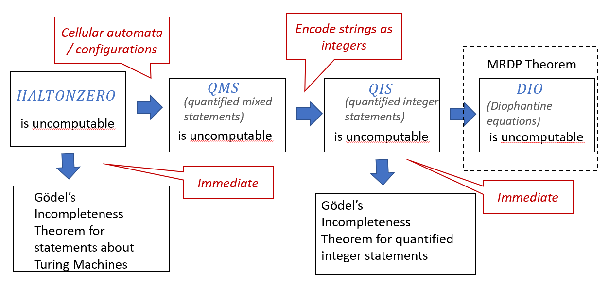
In the rest of this chapter, we will show the proof of Theorem 11.8, following the outline illustrated in Figure 11.1.
Diophantine equations and the MRDP Theorem
Many of the functions people wanted to compute over the years involved solving equations. These have a much longer history than mechanical computers. The Babylonians already knew how to solve some quadratic equations in 2000BC, and the formula for all quadratics appears in the Bakhshali Manuscript that was composed in India around the 3rd century. During the Renaissance, Italian mathematicians discovered generalization of these formulas for cubic and quartic (degrees \(3\) and \(4\)) equations. Many of the greatest minds of the 17th and 18th century, including Euler, Lagrange, Leibniz and Gauss worked on the problem of finding such a formula for quintic equations to no avail, until in the 19th century Ruffini, Abel and Galois showed that no such formula exists, along the way giving birth to group theory.
However, the fact that there is no closed-form formula does not mean we can not solve such equations. People have been solving higher degree equations numerically for ages. The Chinese manuscript Jiuzhang Suanshu from the first century mentions such approaches. Solving polynomial equations is by no means restricted only to ancient history or to students’ homework. The gradient descent method is the workhorse powering many of the machine learning tools that have revolutionized Computer Science over the last several years.
But there are some equations that we simply do not know how to solve by any means. For example, it took more than 200 years until people succeeded in proving that the equation \(a^{11} + b^{11} = c^{11}\) has no solution in integers.3 The notorious difficulty of so called Diophantine equations (i.e., finding integer roots of a polynomial) motivated the mathematician David Hilbert in 1900 to include the question of finding a general procedure for solving such equations in his famous list of twenty-three open problems for mathematics of the 20th century. I don’t think Hilbert doubted that such a procedure exists. After all, the whole history of mathematics up to this point involved the discovery of ever more powerful methods, and even impossibility results such as the inability to trisect an angle with a straightedge and compass, or the non-existence of an algebraic formula for quintic equations, merely pointed out to the need to use more general methods.
Alas, this turned out not to be the case for Diophantine equations. In 1970, Yuri Matiyasevich, building on a decades long line of work by Martin Davis, Hilary Putnam and Julia Robinson, showed that there is simply no method to solve such equations in general:
Let \(\ensuremath{\mathit{DIO}}:\{0,1\}^* \rightarrow \{0,1\}\) be the function that takes as input a string describing a \(100\)-variable polynomial with integer coefficients \(P(x_0,\ldots,x_{99})\) and outputs \(1\) if and only if there exists \(z_0,\ldots,z_{99} \in \N\) s.t. \(P(z_0,\ldots,z_{99})=0\).
Then \(\ensuremath{\mathit{DIO}}\) is uncomputable.
As usual, we assume some standard way to express numbers and text as binary strings. The constant \(100\) is of course arbitrary; the problem is known to be uncomputable even for polynomials of degree four and at most 58 variables. In fact the number of variables can be reduced to nine, at the expense of the polynomial having a larger (but still constant) degree. See Jones’s paper for more about this issue.
The difficulty in finding a way to distinguish between “code” such as NAND-TM programs, and “static content” such as polynomials is just another manifestation of the phenomenon that code is the same as data. While a fool-proof solution for distinguishing between the two is inherently impossible, finding heuristics that do a reasonable job keeps many firewall and anti-virus manufacturers very busy (and finding ways to bypass these tools keeps many hackers busy as well).
Hardness of quantified integer statements
We will not prove the MRDP Theorem (Theorem 11.10). However, as we mentioned, we will prove the uncomputability of \(\ensuremath{\mathit{QIS}}\) (i.e., Theorem 11.9), which is a special case of the MRDP Theorem. The reason is that a Diophantine equation is a special case of a quantified integer statement where the only quantifier is \(\exists\). This means that deciding the truth of quantified integer statements is a potentially harder problem than solving Diophantine equations, and so it is potentially easier to prove that \(\ensuremath{\mathit{QIS}}\) is uncomputable.
If you find the last sentence confusing, it is worthwhile to reread it until you are sure you follow its logic. We are so accustomed to trying to find solutions for problems that it can sometimes be hard to follow the arguments for showing that problems are uncomputable.
Our proof of the uncomputability of \(\ensuremath{\mathit{QIS}}\) (i.e. Theorem 11.9) will, as usual, go by reduction from the Halting problem, but we will do so in two steps:
We will first use a reduction from the Halting problem to show that deciding the truth of quantified mixed statements is uncomputable. Quantified mixed statements involve both strings and integers. Since quantified mixed statements are a more general concept than quantified integer statements, it is easier to prove the uncomputability of deciding their truth.
We will then reduce the problem of quantified mixed statements to quantified integer statements.
Step 1: Quantified mixed statements and computation histories
We define quantified mixed statements as statements involving not just integers and the usual arithmetic operators, but also string variables as well.
A quantified mixed statement is a well-formed statement with no unbound variables involving integers, variables, the operators \(>,<,\times,+,-,=\), the logical operations \(\neg\) (NOT), \(\wedge\) (AND), and \(\vee\) (OR), as well as quantifiers of the form \(\exists_{x\in\N}\), \(\exists_{a\in\{0,1\}^*}\), \(\forall_{y\in\N}\), \(\forall_{b\in\{0,1\}^*}\) where \(x,y,a,b\) are variable names. These also include the operator \(|a|\) which returns the length of a string valued variable \(a\), as well as the operator \(a_i\) where \(a\) is a string-valued variable and \(i\) is an integer valued expression which is true if \(i\) is smaller than the length of \(a\) and the \(i^{th}\) coordinate of \(a\) is \(1\), and is false otherwise.
For example, the true statement that for every string \(a\) there is a string \(b\) that corresponds to \(a\) in reverse order can be phrased as the following quantified mixed statement
Quantified mixed statements are more general than quantified integer statements, and so the following theorem is potentially easier to prove than Theorem 11.9:
Let \(\ensuremath{\mathit{QMS}}:\{0,1\}^* \rightarrow \{0,1\}\) be the function that given a (string representation of) a quantified mixed statement outputs \(1\) if it is true and \(0\) if it is false. Then \(\ensuremath{\mathit{QMS}}\) is uncomputable.
The idea behind the proof is similar to that used in showing that one-dimensional cellular automata are Turing complete (Theorem 8.7) as well as showing that equivalence (or even “fullness”) of context free grammars is uncomputable (Theorem 10.10). We use the notion of a configuration of a NAND-TM program as in Definition 8.8. Such a configuration can be thought of as a string \(\alpha\) over some large-but-finite alphabet \(\Sigma\) describing its current state, including the values of all arrays, scalars, and the index variable i. It can be shown that if \(\alpha\) is the configuration at a certain step of the execution and \(\beta\) is the configuration at the next step, then \(\beta_j = \alpha_j\) for all \(j\) outside of \(\{i-1,i,i+1\}\) where \(i\) is the value of i. In particular, every value \(\beta_j\) is simply a function of \(\alpha_{j-1,j,j+1}\). Using these observations we can write a quantified mixed statement \(\ensuremath{\mathit{NEXT}}(\alpha,\beta)\) that will be true if and only if \(\beta\) is the configuration encoding the next step after \(\alpha\). Since a program \(P\) halts on input \(x\) if and only if there is a sequence of configurations \(\alpha^0,\ldots,\alpha^{t-1}\) (known as a computation history) starting with the initial configuration with input \(x\) and ending in a halting configuration, we can define a quantified mixed statement to determine if there is such a statement by taking a universal quantifier over all strings \(H\) (for history) that encode a tuple \((\alpha^0,\alpha^1,\ldots,\alpha^{t-1})\) and then checking that \(\alpha^0\) and \(\alpha^{t-1}\) are valid starting and halting configurations, and that \(\ensuremath{\mathit{NEXT}}(\alpha^j,\alpha^{j+1})\) is true for every \(j\in \{0,\ldots,t-2\}\).
The proof is obtained by a reduction from the Halting problem. Specifically, we will use the notion of a configuration of a Turing machines (Definition 8.8) that we have seen in the context of proving that one dimensional cellular automata are Turing complete. We need the following facts about configurations:
For every Turing machine \(M\), there is a finite alphabet \(\Sigma\), and a configuration of \(M\) is a string \(\alpha \in \Sigma^*\).
A configuration \(\alpha\) encodes all the state of the program at a particular iteration, including the array, scalar, and index variables.
If \(\alpha\) is a configuration, then \(\beta = \ensuremath{\mathit{NEXT}}_P(\alpha)\) denotes the configuration of the computation after one more iteration. \(\beta\) is a string over \(\Sigma\) of length either \(|\alpha|\) or \(|\alpha|+1\), and every coordinate of \(\beta\) is a function of just three coordinates in \(\alpha\). That is, for every \(j\in \{0,\ldots,|\beta|-1\}\), \(\beta_j = \ensuremath{\mathit{MAP}}_P(\alpha_{j-1},\alpha_j,\alpha_{j+1})\) where \(\ensuremath{\mathit{MAP}}_P:\Sigma^3 \rightarrow \Sigma\) is some function depending on \(P\).
There are simple conditions to check whether a string \(\alpha\) is a valid starting configuration corresponding to an input \(x\), as well as to check whether a string \(\alpha\) is a halting configuration. In particular these conditions can be phrased as quantified mixed statements.
A program \(M\) halts on input \(x\) if and only if there exists a sequence of configurations \(H = (\alpha^0,\alpha^1,\ldots,\alpha^{T-1})\) such that (i) \(\alpha^0\) is a valid starting configuration of \(M\) with input \(x\), (ii) \(\alpha^{T-1}\) is a valid halting configuration of \(P\), and (iii) \(\alpha^{i+1} = \ensuremath{\mathit{NEXT}}_P(\alpha^i)\) for every \(i\in \{0,\ldots,T-2\}\).
We can encode such a sequence \(H\) of configuration as a binary string. For concreteness, we let \(\ell = \lceil \log (|\Sigma|+1) \rceil\) and encode each symbol \(\sigma\) in \(\Sigma \cup \{ ";" \}\) by a string in \(\{0,1\}^\ell\). We use “\(;\)” as a “separator” symbol, and so encode \(H = (\alpha^0,\alpha^1,\ldots,\alpha^{T-1})\) as the concatenation of the encodings of each configuration, using “\(;\)” to separate the encoding of \(\alpha^i\) and \(\alpha^{i+1}\) for every \(i\in [T]\). In particular for every Turing machine \(M\), \(M\) halts on the input \(0\) if and only if the following statement \(\varphi_M\) is true
If we can encode the statement \(\varphi_M\) as a quantified mixed statement then, since \(\varphi_M\) is true if and only if \(\ensuremath{\mathit{HALTONZERO}}(M)=1\), this would reduce the task of computing \(\ensuremath{\mathit{HALTONZERO}}\) to computing \(\ensuremath{\mathit{QMS}}\), and hence imply (using Theorem 9.9 ) that \(\ensuremath{\mathit{QMS}}\) is uncomputable, completing the proof. Indeed, \(\varphi_M\) can be encoded as a quantified mixed statement for the following reasons:
Let \(\alpha,\beta \in \{0,1\}^*\) be two strings that encode configurations of \(M\). We can define a quantified mixed predicate \(\ensuremath{\mathit{NEXT}}(\alpha,\beta)\) that is true if and only if \(\beta = \ensuremath{\mathit{NEXT}}_M(\alpha)\) (i.e., \(\beta\) encodes the configuration obtained by proceeding from \(\alpha\) in one computational step). Indeed \(\ensuremath{\mathit{NEXT}}(\alpha,\beta)\) is true if for every \(i \in \{0,\ldots,|\beta|\}\) which is a multiple of \(\ell\), \(\beta_{i,\ldots,i+\ell-1} = \ensuremath{\mathit{MAP}}_M(\alpha_{i-\ell,\cdots,i+2\ell-1})\) where \(\ensuremath{\mathit{MAP}}_M:\{0,1\}^{3\ell} \rightarrow \{0,1\}^\ell\) is the finite function above (identifying elements of \(\Sigma\) with their encoding in \(\{0,1\}^\ell\)). Since \(\ensuremath{\mathit{MAP}}_M\) is a finite function, we can express it using the logical operations \(\ensuremath{\mathit{AND}}\),\(\ensuremath{\mathit{OR}}\), \(\ensuremath{\mathit{NOT}}\) (for example by computing \(\ensuremath{\mathit{MAP}}_M\) with \(\ensuremath{\mathit{NAND}}\)’s).
Using the above we can now write the condition that for every substring of \(H\) that has the form \(\alpha \ensuremath{\mathit{ENC}}(;) \beta\) with \(\alpha,\beta \in \{0,1\}^\ell\) and \(\ensuremath{\mathit{ENC}}(;)\) being the encoding of the separator “\(;\)”, it holds that \(\ensuremath{\mathit{NEXT}}(\alpha,\beta)\) is true.
Finally, if \(\alpha^0\) is a binary string encoding the initial configuration of \(M\) on input \(0\), checking that the first \(|\alpha^0|\) bits of \(H\) equal \(\alpha_0\) can be expressed using \(\ensuremath{\mathit{AND}}\),\(\ensuremath{\mathit{OR}}\), and \(\ensuremath{\mathit{NOT}}\)’s. Similarly checking that the last configuration encoded by \(H\) corresponds to a state in which \(M\) will halt can also be expressed as a quantified statement.
Together the above yields a computable procedure that maps every Turing machine \(M\) into a quantified mixed statement \(\varphi_M\) such that \(\ensuremath{\mathit{HALTONZERO}}(M)=1\) if and only if \(\ensuremath{\mathit{QMS}}(\varphi_M)=1\). This reduces computing \(\ensuremath{\mathit{HALTONZERO}}\) to computing \(\ensuremath{\mathit{QMS}}\), and hence the uncomputability of \(\ensuremath{\mathit{HALTONZERO}}\) implies the uncomputability of \(\ensuremath{\mathit{QMS}}\).
There are several other ways to show that \(\ensuremath{\mathit{QMS}}\) is uncomputable. For example, we can express the condition that a 1-dimensional cellular automaton eventually writes a “\(1\)” to a given cell from a given initial configuration as a quantified mixed statement over a string encoding the history of all configurations. We can then use the fact that cellular automatons can simulate Turing machines (Theorem 8.7) to reduce the halting problem to \(\ensuremath{\mathit{QMS}}\). We can also use other well known uncomputable problems such as tiling or the post correspondence problem. Exercise 11.5 and Exercise 11.6 explore two alternative proofs of Theorem 11.13.
Step 2: Reducing mixed statements to integer statements
We now show how to prove Theorem 11.9 using Theorem 11.13. The idea is again a proof by reduction. We will show a transformation of every quantified mixed statement \(\varphi\) into a quantified integer statement \(\xi\) that does not use string-valued variables such that \(\varphi\) is true if and only if \(\xi\) is true.
To remove string-valued variables from a statement, we encode every string by a pair integer. We will show that we can encode a string \(x\in \{0,1\}^*\) by a pair of numbers \((X,n)\in \N\) s.t.
\(n=|x|\)
There is a quantified integer statement \(\ensuremath{\mathit{COORD}}(X,i)\) that for every \(i<n\), will be true if \(x_i=1\) and will be false otherwise.
This will mean that we can replace a “for all” quantifier over strings such as \(\forall_{x\in \{0,1\}^*}\) with a pair of quantifiers over integers of the form \(\forall_{X\in \N}\forall_{n\in\N}\) (and similarly replace an existential quantifier of the form \(\exists_{x\in \{0,1\}^*}\) with a pair of quantifiers \(\exists_{X\in \N}\exists_{n\in\N}\)) . We can then replace all calls to \(|x|\) by \(n\) and all calls to \(x_i\) by \(\ensuremath{\mathit{COORD}}(X,i)\). This means that if we are able to define \(\ensuremath{\mathit{COORD}}\) via a quantified integer statement, then we obtain a proof of Theorem 11.9, since we can use it to map every mixed quantified statement \(\varphi\) to an equivalent quantified integer statement \(\xi\) such that \(\xi\) is true if and only if \(\varphi\) is true, and hence \(\ensuremath{\mathit{QMS}}(\varphi)=\ensuremath{\mathit{QIS}}(\xi)\). Such a procedure implies that the task of computing \(\ensuremath{\mathit{QMS}}\) reduces to the task of computing \(\ensuremath{\mathit{QIS}}\), which means that the uncomputability of \(\ensuremath{\mathit{QMS}}\) implies the uncomputability of \(\ensuremath{\mathit{QIS}}\).
The above shows that proof of Theorem 11.9 all boils down to finding the right encoding of strings as integers, and the right way to implement \(\ensuremath{\mathit{COORD}}\) as a quantified integer statement. To achieve this we use the following technical result :
There is a sequence of prime numbers \(p_0 < p_1 < p_2 < \cdots\) such that there is a quantified integer statement \(\ensuremath{\mathit{PSEQ}}(p,i)\) that is true if and only if \(p=p_i\).
Using Lemma 11.15 we can encode a \(x\in\{0,1\}^*\) by the numbers \((X,n)\) where \(X = \prod_{x_i=1} p_i\) and \(n=|x|\). We can then define the statement \(\ensuremath{\mathit{COORD}}(X,i)\) as
Thus all that is left to conclude the proof of Theorem 11.9 is to prove Lemma 11.15, which we now proceed to do.
The sequence of prime numbers we consider is the following: We fix \(C\) to be a sufficiently large constant (\(C=2^{2^{34}}\) will do) and define \(p_i\) to be the smallest prime number that is in the interval \([(i+C)^3+1,(i+C+1)^3-1]\). It is known that there exists such a prime number for every \(i\in\N\). Given this, the definition of \(\ensuremath{\mathit{PSEQ}}(p,i)\) is simple:
To sum up we have shown that for every quantified mixed statement \(\varphi\), we can compute a quantified integer statement \(\xi\) such that \(\ensuremath{\mathit{QMS}}(\varphi)=1\) if and only if \(\ensuremath{\mathit{QIS}}(\xi)=1\). Hence the uncomputability of \(\ensuremath{\mathit{QMS}}\) (Theorem 11.13) implies the uncomputability of \(\ensuremath{\mathit{QIS}}\), completing the proof of Theorem 11.9, and so also the proof of Gödel’s Incompleteness Theorem for quantified integer statements (Theorem 11.8).
- Uncomputable functions include also functions that seem to have nothing to do with NAND-TM programs or other computational models such as determining the satisfiability of Diophantine equations.
- This also implies that for any sound proof system (and in particular every finite axiomatic system) \(S\), there are interesting statements \(X\) (namely of the form “\(F(x)=0\)” for an uncomputable function \(F\)) such that \(S\) is not able to prove either \(X\) or its negation.
Exercises
Prove Theorem 11.8 using Theorem 11.9.
Let \(\ensuremath{\mathit{FINDPROOF}}:\{0,1\}^* \rightarrow \{0,1\}\) be the following function. On input a Turing machine \(V\) (which we think of as the verifying algorithm for a proof system) and a string \(x\in \{0,1\}^*\), \(\ensuremath{\mathit{FINDPROOF}}(V,x)=1\) if and only if there exists \(w\in \{0,1\}^*\) such that \(V(x,w)=1\).
Prove that \(\ensuremath{\mathit{FINDPROOF}}\) is uncomputable.
Prove that there exists a Turing machine \(V\) such that \(V\) halts on every input \(x,v\) but the function \(\ensuremath{\mathit{FINDPROOF}}_V\) defined as \(\ensuremath{\mathit{FINDPROOF}}_V(x) = \ensuremath{\mathit{FINDPROOF}}(V,x)\) is uncomputable. See footnote for hint.4
Let \(\ensuremath{\mathit{FSQRT}}(n,m) = \forall_{j \in \N} ((j \times j)>m) \vee (j \leq n)\). Prove that \(\ensuremath{\mathit{FSQRT}}(n,m)\) is true if and only if \(n =\floor{\sqrt{m}}\).
For every representation of logical statements as strings, we can define an axiomatic proof system to consist of a finite set of strings \(A\) and a finite set of rules \(I_0,\ldots,I_{m-1}\) with \(I_j: (\{0,1\}^*)^{k_j} \rightarrow \{0,1\}^*\) such that a proof \((s_1,\ldots,s_n)\) that \(s_n\) is true is valid if for every \(i\), either \(s_i \in A\) or is some \(j\in [m]\) and are \(i_1,\ldots,i_{k_j} < i\) such that \(s_i = I_j(s_{i_1},\ldots,i_{k_j})\). A system is sound if whenever there is no false \(s\) such that there is a proof that \(s\) is true. Prove that for every uncomputable function \(F:\{0,1\}^* \rightarrow \{0,1\}\) and every sound axiomatic proof system \(S\) (that is characterized by a finite number of axioms and inference rules), there is some input \(x\) for which the proof system \(S\) is not able to prove neither that \(F(x)=0\) nor that \(F(x) \neq 0\).
In the Post Correspondence Problem the input is a set \(S = \{ (\alpha^0,\beta^0), \ldots, (\beta^{c-1},\beta^{c-1}) \}\) where each \(\alpha^i\) and \(\beta^j\) is a string in \(\{0,1\}^*\). We say that \(\ensuremath{\mathit{PCP}}(S)=1\) if and only if there exists a list \((\alpha_0,\beta_0),\ldots,(\alpha_{m-1},\beta_{m-1})\) of pairs in \(S\) such that
Use this fact to provide a direct proof that \(\ensuremath{\mathit{QMS}}\) is uncomputable by showing that there exists a computable map \(R:\{0,1\}^* \rightarrow \{0,1\}^*\) such that \(\ensuremath{\mathit{PCP}}(S) = \ensuremath{\mathit{QMS}}(R(S))\) for every string \(S\) encoding an instance of the post correspondence problem.
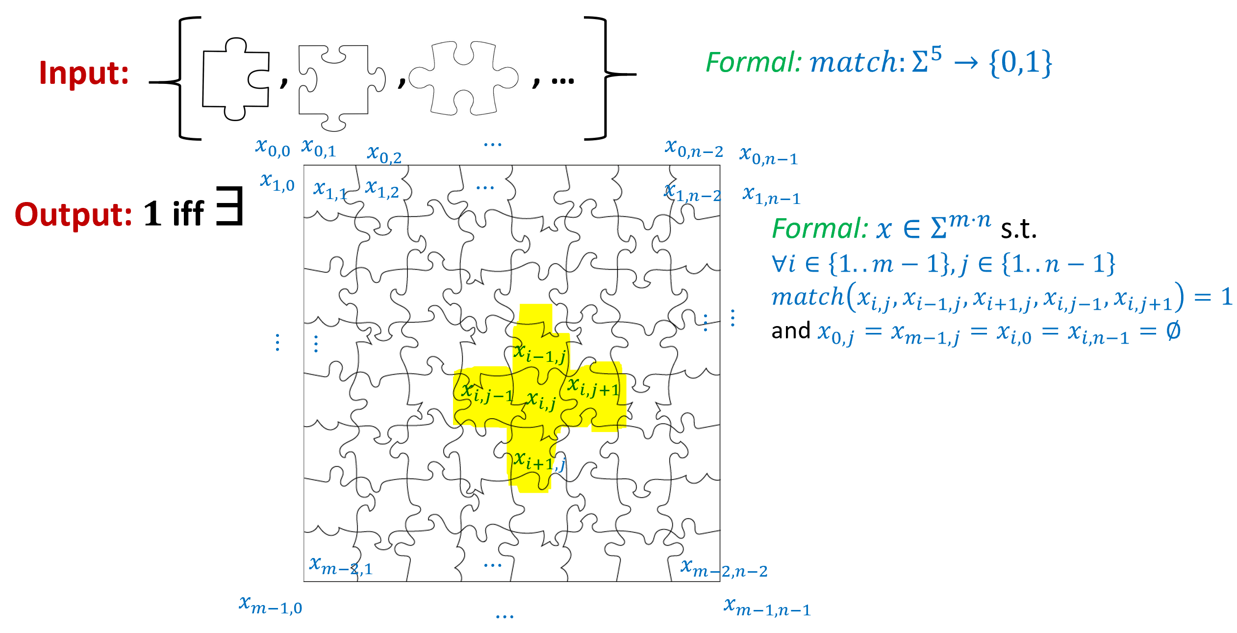
Let \(\ensuremath{\mathit{PUZZLE}}:\{0,1\}^* \rightarrow \{0,1\}\) be the problem of determining, given a finite collection of types of “puzzle pieces”, whether it is possible to put them together in a rectangle, see Figure 11.3. Formally, we think of such a collection as a finite set \(\Sigma\) (see Figure 11.3). We model the criteria as to which pieces “fit together” by a pair of finite function \(match_{\updownarrow}, match_{\leftrightarrow}:\Sigma^2 \rightarrow \{0,1\}\) such that a piece \(a\) fits above a piece \(b\) if and only if \(match_{\updownarrow}(a,b)=1\) and a piece \(c\) fits to the left of a piece \(d\) if and only if \(match_{\leftrightarrow}(c,d)=1\). To model the “straight edge” pieces that can be placed next to a “blank spot” we assume that \(\Sigma\) contains the symbol \(\varnothing\) and the matching functions are defined accordingly. A square tiling of \(\Sigma\) is an \(m\times n\) long string \(x \in \Sigma^{mn}\), such that for every \(i\in \{1,\ldots,m-2 \}\) and \(j\in \{1,\ldots,n-2 \}\), \(match(x_{i,j},x_{i-1,j},x_{i+1,j},x_{i,j-1},x_{i,j+1})=1\) (i.e., every “internal pieve” fits in with the pieces adjacent to it). We also require all of the “outer pieces” (i.e., \(x_{i,j}\) where \(i\in \{0,m-1\}\) of \(j\in \{0,n-1\}\)) are “blank” or equal to \(\varnothing\). The function \(\ensuremath{\mathit{PUZZLE}}\) takes as input a string describing the set \(\Sigma\) and the function \(match\) and outputs \(1\) if and only if there is some square tiling of \(\Sigma\): some not all blank string \(x\in \Sigma^{mn}\) satisfying the above condition.
Prove that \(\ensuremath{\mathit{PUZZLE}}\) is uncomputable.
Give a reduction from \(\ensuremath{\mathit{PUZZLE}}\) to \(\ensuremath{\mathit{QMS}}\).
The MRDP theorem states that the problem of determining, given a \(k\)-variable polynomial \(p\) with integer coefficients, whether there exists integers \(x_0,\ldots,x_{k-1}\) such that \(p(x_0,\ldots,x_{k-1})=0\) is uncomputable. Consider the following quadratic integer equation problem: the input is a list of polynomials \(p_0,\ldots,p_{m-1}\) over \(k\) variables with integer coefficients, where each of the polynomials is of degree at most two (i.e., it is a quadratic function). The goal is to determine whether there exist integers \(x_0,\ldots,x_{k-1}\) that solve the equations \(p_0(x)= \cdots = p_{m-1}(x)=0\).
Use the MRDP Theorem to prove that this problem is uncomputable. That is, show that the function \(\ensuremath{\mathit{QUADINTEQ}}:\{0,1\}^* \rightarrow \{0,1\}\) is uncomputable, where this function gets as input a string describing the polynomials \(p_0,\ldots,p_{m-1}\) (each with integer coefficients and degree at most two), and outputs \(1\) if and only if there exists \(x_0,\ldots,x_{k-1} \in \mathbb{Z}\) such that for every \(i\in [m]\), \(p_i(x_0,\ldots,x_{k-1})=0\). See footnote for hint5
In this question we define the NAND-TM variant of the busy beaver function.
We define the function \(T:\{0,1\}^* \rightarrow \mathbb{N}\) as follows: for every string \(P\in \{0,1\}^*\), if \(P\) represents a NAND-TM program such that when \(P\) is executed on the input \(0\) (i.e., the string of length 1 that is simply \(0\)), a total of \(M\) lines are executed before the program halts, then \(T(P)=M\). Otherwise (if \(P\) does not represent a NAND-TM program, or it is a program that does not halt on \(0\)), \(T(P)=0\). Prove that \(T\) is uncomputable.
Let \(\ensuremath{\mathit{TOWER}}(n)\) denote the number \(\underbrace{2^{2^{2^{{\cdots}^2}}}}_{n\text{ times}}\) (that is, a “tower of powers of two” of height \(n\)). To get a sense of how fast this function grows, \(\ensuremath{\mathit{TOWER}}(1)=2\), \(\ensuremath{\mathit{TOWER}}(2)=2^2=4\), \(\ensuremath{\mathit{TOWER}}(3)=2^{2^2}=16\), \(\ensuremath{\mathit{TOWER}}(4) = 2^{16} = 65536\) and \(\ensuremath{\mathit{TOWER}}(5) = 2^{65536}\) which is about \(10^{20000}\). \(\ensuremath{\mathit{TOWER}}(6)\) is already a number that is too big to write even in scientific notation. Define \(\ensuremath{\mathit{NBB}}:\mathbb{N} \rightarrow \mathbb{N}\) (for “NAND-TM Busy Beaver”) to be the function \(\ensuremath{\mathit{NBB}}(n) = \max_{P\in \{0,1\}^n} T(P)\) where \(T:\mathbb{N} \rightarrow \mathbb{N}\) is the function defined in Item 1. Prove that \(\ensuremath{\mathit{NBB}}\) grows faster than \(\ensuremath{\mathit{TOWER}}\), in the sense that \(\ensuremath{\mathit{TOWER}}(n) = o(\ensuremath{\mathit{NBB}}(n))\) (i.e., for every \(\epsilon>0\), there exists \(n_0\) such that for every \(n>n_0\), \(\ensuremath{\mathit{TOWER}}(n) < \epsilon \cdot \ensuremath{\mathit{NBB}}(n)\).).6
Bibliographical notes
As mentioned before, Gödel, Escher, Bach (Hofstadter, 1999) is a highly recommended book covering Gödel’s Theorem. A classic popular science book about Fermat’s Last Theorem is (Singh, 1997) .
Cantor’s are used for both Turing and Gödel’s theorems. In a twist of fate, using techniques originating from the works of Gödel and Turing, Paul Cohen showed in 1963 that Cantor’s Continuum Hypothesis is independent of the axioms of set theory, which means that neither it nor its negation is provable from these axioms and hence in some sense can be considered as “neither true nor false” (see (Cohen, 2008) ). The Continuum Hypothesis is the conjecture that for every subset \(S\) of \(\mathbb{R}\), either there is a one-to-one and onto map between \(S\) and \(\N\) or there is a one-to-one and onto map between \(S\) and \(\mathbb{R}\). It was conjectured by Cantor and listed by Hilbert in 1900 as one of the most important problems in mathematics. See also the non-conventional survey of Shelah (Shelah, 2003) . See here for recent progress on a related question.
Thanks to Alex Lombardi for pointing out an embarrassing mistake in the description of Fermat’s Last Theorem. (I said that it was open for exponent 11 before Wiles’ work.)
- ↩
This happens to be a false statement.
- ↩
It is unknown whether this statement is true or false.
- ↩
This is a special case of what’s known as “Fermat’s Last Theorem” which states that \(a^n + b^n = c^n\) has no solution in integers for \(n>2\). This was conjectured in 1637 by Pierre de Fermat but only proven by Andrew Wiles in 1991. The case \(n=11\) (along with all other so called “regular prime exponents”) was established by Kummer in 1850.
- ↩
Hint: think of \(x\) as saying “Turing machine \(M\) halts on input \(u\)” and \(w\) being a proof that is the number of steps that it will take for this to happen. Can you find an always-halting \(V\) that will verify such statements?
- ↩
You can replace the equation \(y=x^4\) with the pair of equations \(y=z^2\) and \(z=x^2\). Also, you can replace the equation \(w = x^6\) with the three equations \(w=yu\), \(y = x^4\) and \(u=x^2\).
- ↩
You will not need to use very specific properties of the \(\ensuremath{\mathit{TOWER}}\) function in this exercise. For example, \(\ensuremath{\mathit{NBB}}(n)\) also grows faster than the Ackerman function. You might find Aaronson’s blog post on the same topic to be quite interesting, and relevant to this book at large. If you like it then you might also enjoy this piece by Terence Tao.
Comments
Comments are posted on the GitHub repository using the utteranc.es app. A GitHub login is required to comment. If you don't want to authorize the app to post on your behalf, you can also comment directly on the GitHub issue for this page.
Compiled on 12/06/2023 00:07:25
Copyright 2023, Boaz Barak.

This work is
licensed under a Creative Commons
Attribution-NonCommercial-NoDerivatives 4.0 International License.
Produced using pandoc and panflute with templates derived from gitbook and bookdown.