See any bugs/typos/confusing explanations? Open a GitHub issue. You can also comment below

★ See also the PDF version of this chapter (better formatting/references) ★

Restricted computational models

See that Turing completeness is not always a good thing.
Another example of an always-halting formalism: context-free grammars and simply typed $\lambda$ calculus.
The pumping lemma for non context-free functions.
Examples of computable and uncomputable semantic properties of regular expressions and context-free grammars.

“Happy families are all alike; every unhappy family is unhappy in its own way”, Leo Tolstoy (opening of the book “Anna Karenina”).

We have seen that many models of computation are Turing equivalent, including Turing machines, NAND-TM/NAND-RAM programs, standard programming languages such as C/Python/Javascript, as well as other models such as the $\lambda$ calculus and even the game of life. The flip side of this is that for all these models, Rice’s theorem (Theorem 9.15) holds as well, which means that any semantic property of programs in such a model is uncomputable.

The uncomputability of halting and other semantic specification problems for Turing equivalent models motivates restricted computational models that are (a) powerful enough to capture a set of functions useful for certain applications but (b) weak enough that we can still solve semantic specification problems on them. In this chapter we discuss several such examples.

We can use restricted computational models to bypass limitations such as uncomputability of the Halting problem and Rice’s Theorem. Such models can compute only a restricted subclass of functions, but allow to answer at least some semantic questions on programs.

10.1: Some restricted computational models. We have already seen two equivalent restricted models of computation: regular expressions and deterministic finite automata. We show a more powerful model: context-free grammars. We also present tools to demonstrate that some functions *can not* be computed in these models.

Turing completeness as a bug

We have seen that seemingly simple computational models or systems can turn out to be Turing complete. The following webpage lists several examples of formalisms that “accidentally” turned out to Turing complete, including supposedly limited languages such as the C preprocessor, CSS, (certain variants of) SQL, sendmail configuration, as well as games such as Minecraft, Super Mario, and the card game “Magic: The Gathering”. Turing completeness is not always a good thing, as it means that such formalisms can give rise to arbitrarily complex behavior. For example, the postscript format (a precursor of PDF) is a Turing-complete programming language meant to describe documents for printing. The expressive power of postscript can allow for short descriptions of very complex images, but it also gave rise to some nasty surprises, such as the attacks described in this page ranging from using infinite loops as a denial of service attack, to accessing the printer’s file system.

An interesting recent example of the pitfalls of Turing-completeness arose in the context of the cryptocurrency Ethereum. The distinguishing feature of this currency is the ability to design “smart contracts” using an expressive (and in particular Turing-complete) programming language. In our current “human operated” economy, Alice and Bob might sign a contract to agree that if condition X happens then they will jointly invest in Charlie’s company. Ethereum allows Alice and Bob to create a joint venture where Alice and Bob pool their funds together into an account that will be governed by some program $P$ that decides under what conditions it disburses funds from it. For example, one could imagine a piece of code that interacts between Alice, Bob, and some program running on Bob’s car that allows Alice to rent out Bob’s car without any human intervention or overhead.

Specifically Ethereum uses the Turing-complete programming language solidity which has a syntax similar to JavaScript. The flagship of Ethereum was an experiment known as The “Decentralized Autonomous Organization” or The DAO. The idea was to create a smart contract that would create an autonomously run decentralized venture capital fund, without human managers, where shareholders could decide on investment opportunities. The DAO was at the time the biggest crowdfunding success in history. At its height the DAO was worth 150 million dollars, which was more than ten percent of the total Ethereum market. Investing in the DAO (or entering any other “smart contract”) amounts to providing your funds to be run by a computer program. i.e., “code is law”, or to use the words the DAO described itself: “The DAO is borne from immutable, unstoppable, and irrefutable computer code”. Unfortunately, it turns out that (as we saw in Chapter 9) understanding the behavior of computer programs is quite a hard thing to do. A hacker (or perhaps, some would say, a savvy investor) was able to fashion an input that caused the DAO code to enter into an infinite recursive loop in which it continuously transferred funds into the hacker’s account, thereby cleaning out about 60 million dollars out of the DAO. While this transaction was “legal” in the sense that it complied with the code of the smart contract, it was obviously not what the humans who wrote this code had in mind. The Ethereum community struggled with the response to this attack. Some tried the “Robin Hood” approach of using the same loophole to drain the DAO funds into a secure account, but it only had limited success. Eventually, the Ethereum community decided that the code can be mutable, stoppable, and refutable. Specifically, the Ethereum maintainers and miners agreed on a “hard fork” (also known as a “bailout”) to revert history to before the hacker’s transaction occurred. Some community members strongly opposed this decision, and so an alternative currency called Ethereum Classic was created that preserved the original history.

Context free grammars

If you have ever written a program, you’ve experienced a syntax error. You probably also had the experience of your program entering into an infinite loop. What is less likely is that the compiler or interpreter entered an infinite loop while trying to figure out if your program has a syntax error.

When a person designs a programming language, they need to determine its syntax. That is, the designer decides which strings corresponds to valid programs, and which ones do not (i.e., which strings contain a syntax error). To ensure that a compiler or interpreter always halts when checking for syntax errors, language designers typically do not use a general Turing-complete mechanism to express their syntax. Rather they use a restricted computational model. One of the most popular choices for such models is context free grammars.

To explain context free grammars, let us begin with a canonical example. Consider the function $\ensuremath{\mathit{ARITH}}:\Sigma^* \rightarrow \{0,1\}$ that takes as input a string $x$ over the alphabet $\Sigma = \{ (,),+,-,\times,\div,0,1,2,3,4,5,6,7,8,9\}$ and returns $1$ if and only if the string $x$ represents a valid arithmetic expression. Intuitively, we build expressions by applying an operation such as $+$,$-$,$\times$ or $\div$ to smaller expressions, or enclosing them in parentheses, where the “base case” corresponds to expressions that are simply numbers. More precisely, we can make the following definitions:

A digit is one of the symbols $0,1,2,3,4,5,6,7,8,9$.
A number is a sequence of digits. (For simplicity we drop the condition that the sequence does not have a leading zero, though it is not hard to encode it in a context-free grammar as well.)
An operation is one of $+,-,\times,\div$
An expression has either the form “number”, the form “sub-expression1 operation sub-expression2”, or the form “(sub-expression1)”, where “sub-expression1” and “sub-expression2” are themselves expressions. (Note that this is a recursive definition.)

A context free grammar (CFG) is a formal way of specifying such conditions. A CFG consists of a set of rules that tell us how to generate strings from smaller components. In the above example, one of the rules is “if $exp1$ and $exp2$ are valid expressions, then $exp1 \times exp2$ is also a valid expression”; we can also write this rule using the shorthand $expression \; \Rightarrow \; expression \; \times \; expression$. As in the above example, the rules of a context-free grammar are often recursive: the rule $expression \; \Rightarrow\; expression \; \times \; expression$ defines valid expressions in terms of itself. We now formally define context-free grammars:

Let $\Sigma$ be some finite set. A context free grammar (CFG) over $\Sigma$ is a triple $(V,R,s)$ such that:

$V$, known as the variables, is a set disjoint from $\Sigma$.
$s\in V$ is known as the initial variable.
$R$ is a set of rules. Each rule is a pair $(v,z)$ with $v\in V$ and $z\in (\Sigma \cup V)^*$. We often write the rule $(v,z)$ as $v \Rightarrow z$ and say that the string $z$ can be derived from the variable $v$.

The example above of well-formed arithmetic expressions can be captured formally by the following context free grammar:

The alphabet $\Sigma$ is $\{ (,),+,-,\times,\div,0,1,2,3,4,5,6,7,8,9\}$
The variables are $V = \{ expression \;,\; number \;,\; digit \;,\; operation \}$.
The rules are the set $R$ containing the following $19$ rules:
- The $4$ rules $operation \Rightarrow +$, $operation \Rightarrow -$, $operation \Rightarrow \times$, and $operation \Rightarrow \div$.
- The $10$ rules $digit \Rightarrow 0$,$\ldots$, $digit \Rightarrow 9$.
- The rule $number \Rightarrow digit$.
- The rule $number \Rightarrow digit\; number$.
- The rule $expression \Rightarrow number$.
- The rule $expression \Rightarrow expression \; operation \; expression$.
- The rule $expression \Rightarrow (expression)$.
The starting variable is $expression$

People use many different notations to write context free grammars. One of the most common notations is the Backus–Naur form. In this notation we write a rule of the form $v \Rightarrow a$ (where $v$ is a variable and $a$ is a string) in the form <v> := a. If we have several rules of the form $v \mapsto a$, $v \mapsto b$, and $v \mapsto c$ then we can combine them as <v> := a|b|c. (In words we say that $v$ can derive either $a$, $b$, or $c$.) For example, the Backus-Naur description for the context free grammar of Example 10.3 is the following (using ASCII equivalents for operations):

operation  := +|-|*|/
digit      := 0|1|2|3|4|5|6|7|8|9
number     := digit|digit number
expression := number|expression operation expression|(expression)

Another example of a context free grammar is the “matching parentheses” grammar, which can be represented in Backus-Naur as follows:

match  := ""|match match|(match)

A string over the alphabet $\{$ (,) $\}$ can be generated from this grammar (where match is the starting expression and "" corresponds to the empty string) if and only if it consists of a matching set of parentheses. In contrast, by Lemma 6.20 there is no regular expression that matches a string $x$ if and only if $x$ contains a valid sequence of matching parentheses.

Context-free grammars as a computational model

We can think of a context-free grammar over the alphabet $\Sigma$ as defining a function that maps every string $x$ in $\Sigma^*$ to $1$ or $0$ depending on whether $x$ can be generated by the rules of the grammars. We now make this definition formally.

If $G=(V,R,s)$ is a context-free grammar over $\Sigma$, then for two strings $\alpha,\beta \in (\Sigma \cup V)^*$ we say that $\beta$ can be derived in one step from $\alpha$, denoted by $\alpha \Rightarrow_G \beta$, if we can obtain $\beta$ from $\alpha$ by applying one of the rules of $G$. That is, we obtain $\beta$ by replacing in $\alpha$ one occurrence of the variable $v$ with the string $z$, where $v \Rightarrow z$ is a rule of $G$.

We say that $\beta$ can be derived from $\alpha$, denoted by $\alpha \Rightarrow_G^* \beta$, if it can be derived by some finite number $k$ of steps. That is, if there are $\alpha_1,\ldots,\alpha_{k-1} \in (\Sigma \cup V)^*$, so that $\alpha \Rightarrow_G \alpha_1 \Rightarrow_G \alpha_2 \Rightarrow_G \cdots \Rightarrow_G \alpha_{k-1} \Rightarrow_G \beta$.

We say that $x\in \Sigma^*$ is matched by $G=(V,R,s)$ if $x$ can be derived from the starting variable $s$ (i.e., if $s \Rightarrow_G^* x$). We define the function computed by $(V,R,s)$ to be the map $\Phi_{V,R,s}:\Sigma^* \rightarrow \{0,1\}$ such that $\Phi_{V,R,s}(x)=1$ iff $x$ is matched by $(V,R,s)$. A function $F:\Sigma^* \rightarrow \{0,1\}$ is context free if $F = \Phi_{V,R,s}$ for some CFG $(V,R,s)$.¹

A priori it might not be clear that the map $\Phi_{V,R,s}$ is computable, but it turns out that this is the case.

For every CFG $(V,R,s)$ over $\{0,1\}$, the function $\Phi_{V,R,s}:\{0,1\}^* \rightarrow \{0,1\}$ is computable.

As usual we restrict attention to grammars over $\{0,1\}$ although the proof extends to any finite alphabet $\Sigma$.

We only sketch the proof. We start with the observation we can convert every CFG to an equivalent version of Chomsky normal form, where all rules either have the form $u \rightarrow vw$ for variables $u,v,w$ or the form $u \rightarrow \sigma$ for a variable $u$ and symbol $\sigma \in \Sigma$, plus potentially the rule $s \rightarrow \ensuremath{\text{\texttt{""}}}$ where $s$ is the starting variable.

The idea behind such a transformation is to simply add new variables as needed, and so for example we can translate a rule such as $v \rightarrow u\sigma w$ into the three rules $v \rightarrow ur$, $r \rightarrow tw$ and $t \rightarrow \sigma$.

Using the Chomsky Normal form we get a natural recursive algorithm for computing whether $s \Rightarrow_G^* x$ for a given grammar $G$ and string $x$. We simply try all possible guesses for the first rule $s \rightarrow uv$ that is used in such a derivation, and then all possible ways to partition $x$ as a concatenation $x=x'x''$. If we guessed the rule and the partition correctly, then this reduces our task to checking whether $u \Rightarrow_G^* x'$ and $v \Rightarrow_G^* x''$, which (as it involves shorter strings) can be done recursively. The base cases are when $x$ is empty or a single symbol, and can be easily handled.

While we focus on the task of deciding whether a CFG matches a string, the algorithm to compute $\Phi_{V,R,s}$ actually gives more information than that. That is, on input a string $x$, if $\Phi_{V,R,s}(x)=1$ then the algorithm yields the sequence of rules that one can apply from the starting vertex $s$ to obtain the final string $x$. We can think of these rules as determining a tree with $s$ being the root vertex and the sinks (or leaves) corresponding to the substrings of $x$ that are obtained by the rules that do not have a variable in their second element. This tree is known as the parse tree of $x$, and often yields very useful information about the structure of $x$.

Often the first step in a compiler or interpreter for a programming language is a parser that transforms the source into the parse tree (also known as the abstract syntax tree). There are also tools that can automatically convert a description of a context-free grammars into a parser algorithm that computes the parse tree of a given string. (Indeed, the above recursive algorithm can be used to achieve this, but there are much more efficient versions, especially for grammars that have particular forms, and programming language designers often try to ensure their languages have these more efficient grammars.)

The power of context free grammars

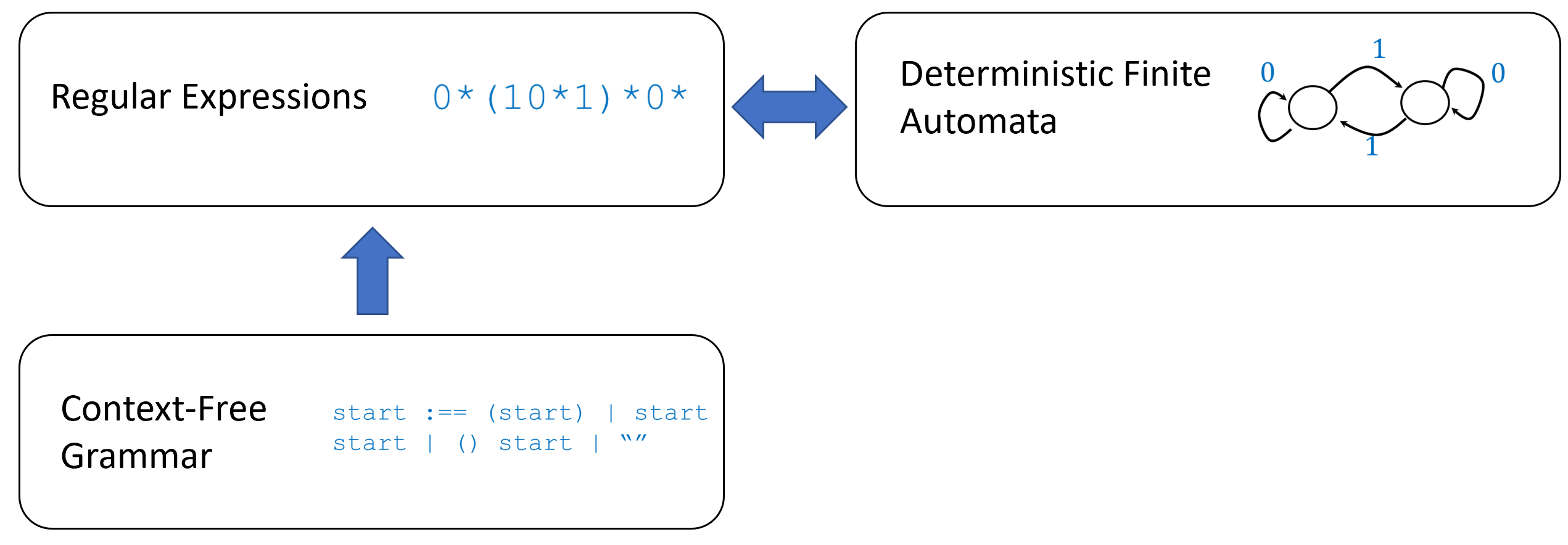
Context free grammars can capture every regular expression:

Let $e$ be a regular expression over $\{0,1\}$, then there is a CFG $(V,R,s)$ over $\{0,1\}$ such that $\Phi_{V,R,s}=\Phi_{e}$.

We prove the theorem by induction on the length of $e$. If $e$ is an expression of one bit length, then $e=0$ or $e=1$, in which case we leave it to the reader to verify that there is a (trivial) CFG that computes it. Otherwise, we fall into one of the following case: case 1: $e = e'e''$, case 2: $e = e'|e''$ or case 3: $e=(e')^*$ where in all cases $e',e''$ are shorter regular expressions. By the induction hypothesis, we can define grammars $(V',R',s')$ and $(V'',R'',s'')$ that compute $\Phi_{e'}$ and $\Phi_{e''}$ respectively. By renaming variables, we can also assume without loss of generality that $V'$ and $V''$ are disjoint.

In case 1, we can define the new grammar as follows: we add a new starting variable $s \not\in V \cup V'$ and the rule $s \mapsto s's''$. In case 2, we can define the new grammar as follows: we add a new starting variable $s \not\in V \cup V'$ and the rules $s \mapsto s'$ and $s \mapsto s''$. Case 3 will be the only one that uses recursion. As before we add a new starting variable $s \not\in V \cup V'$, but now add the rules $s \mapsto \ensuremath{\text{\texttt{""}}}$ (i.e., the empty string) and also add, for every rule of the form $(s',\alpha) \in R'$, the rule $s \mapsto s\alpha$ to $R$.

We leave it to the reader as (a very good!) exercise to verify that in all three cases the grammars we produce capture the same function as the original expression.

It turns out that CFG’s are strictly more powerful than regular expressions. In particular, as we’ve seen, the “matching parentheses” function $\ensuremath{\mathit{MATCHPAREN}}$ can be computed by a context free grammar, whereas, as shown in Lemma 6.20, it cannot be computed by regular expressions. Here is another example:

Let $\ensuremath{\mathit{PAL}}:\{0,1,;\}^* \rightarrow \{0,1\}$ be the function defined in Solved Exercise 6.4 where $\ensuremath{\mathit{PAL}}(w)=1$ iff $w$ has the form $u;u^R$. Then $\ensuremath{\mathit{PAL}}$ can be computed by a context-free grammar

A simple grammar computing $\ensuremath{\mathit{PAL}}$ can be described using Backus–Naur notation:

start      := ; | 0 start 0 | 1 start 1

One can prove by induction that this grammar generates exactly the strings $w$ such that $\ensuremath{\mathit{PAL}}(w)=1$.

A more interesting example is computing the strings of the form $u;v$ that are not palindromes:

Prove that there is a context free grammar that computes $\ensuremath{\mathit{NPAL}}:\{0,1,;\}^* \rightarrow \{0,1\}$ where $\ensuremath{\mathit{NPAL}}(w)=1$ if $w=u;v$ but $v \neq u^R$.

Using Backus–Naur notation we can describe such a grammar as follows

palindrome      := ; | 0 palindrome 0 | 1 palindrome 1
different       := 0 palindrome 1 | 1 palindrome 0
start           := different | 0 start | 1 start | start 0 | start 1

In words, this means that we can characterize a string $w$ such that $\ensuremath{\mathit{NPAL}}(w)=1$ as having the following form

\[ w = \alpha b u ; u^R b' \beta \]

where $\alpha,\beta,u$ are arbitrary strings and $b \neq b'$. Hence we can generate such a string by first generating a palindrome $u; u^R$ (palindrome variable), then adding $0$ on either the left or right and $1$ on the opposite side to get something that is not a palindrome (different variable), and then we can add arbitrary number of $0$’s and $1$’s on either end (the start variable).

Limitations of context-free grammars (optional)

Even though context-free grammars are more powerful than regular expressions, there are some simple languages that are not captured by context free grammars. One tool to show this is the context-free grammar analog of the “pumping lemma” (Theorem 6.21):

Let $(V,R,s)$ be a CFG over $\Sigma$, then there is some numbers $n_0,n_1 \in \N$ such that for every $x \in \Sigma^*$ with $|x|>n_0$, if $\Phi_{V,R,s}(x)=1$ then $x=abcde$ such that $|b|+|c|+|d| \leq n_1$, $|b|+|d| \geq 1$, and $\Phi_{V,R,s}(ab^kcd^ke)=1$ for every $k\in \N$.

The context-free pumping lemma is even more cumbersome to state than its regular analog, but you can remember it as saying the following: “If a long enough string is matched by a grammar, there must be a variable that is repeated in the derivation.”

We only sketch the proof. The idea is that if the total number of symbols in the rules of the grammar is $n_0$, then the only way to get $|x|>n_0$ with $\Phi_{V,R,s}(x)=1$ is to use recursion. That is, there must be some variable $v \in V$ such that we are able to derive from $v$ the value $bvd$ for some strings $b,d \in \Sigma^*$, and then further on derive from $v$ some string $c\in \Sigma^*$ such that $bcd$ is a substring of $x$ (in other words, $x=abcde$ for some $a,e \in \{0,1\}^*$). If we take the variable $v$ satisfying this requirement with a minimum number of derivation steps, then we can ensure that $|bcd|$ is at most some constant depending on $n_0$ and we can set $n_1$ to be that constant ($n_1=10 \cdot |R| \cdot n_0$ will do, since we will not need more than $|R|$ applications of rules, and each such application can grow the string by at most $n_0$ symbols).

Thus by the definition of the grammar, we can repeat the derivation to replace the substring $bcd$ in $x$ with $b^kcd^k$ for every $k\in \N$ while retaining the property that the output of $\Phi_{V,R,s}$ is still one. Since $bcd$ is a substring of $x$, we can write $x=abcde$ and are guaranteed that $ab^kcd^ke$ is matched by the grammar for every $k$.

Using Theorem 10.8 one can show that even the simple function $F:\{0,1\}^* \rightarrow \{0,1\}$ defined as follows:

\[F(x) = \begin{cases}1 & x =ww \text{ for some } w\in \{0,1\}^* \\ 0 & \text{otherwise} \end{cases}\]

is not context free. (In contrast, the function $G:\{0,1\}^* \rightarrow \{0,1\}$ defined as $G(x)=1$ iff $x=w_0w_1\cdots w_{n-1}w_{n-1}w_{n-2}\cdots w_0$ for some $w\in \{0,1\}^*$ and $n=|w|$ is context free, can you see why?.)

Let $\ensuremath{\mathit{EQ}}:\{0,1,;\}^* \rightarrow \{0,1\}$ be the function such that $\ensuremath{\mathit{EQ}}(x)=1$ if and only if $x=u;u$ for some $u\in \{0,1\}^*$. Then $\ensuremath{\mathit{EQ}}$ is not context free.

We use the context-free pumping lemma. Suppose towards the sake of contradiction that there is a grammar $G$ that computes $\ensuremath{\mathit{EQ}}$, and let $n_0$ be the constant obtained from Theorem 10.8.

Consider the string $x= 1^{n_0}0^{n_0};1^{n_0}0^{n_0}$, and write it as $x=abcde$ as per Theorem 10.8, with $|bcd| \leq n_0$ and with $|b|+|d| \geq 1$. By Theorem 10.8, it should hold that $\ensuremath{\mathit{EQ}}(ace)=1$. However, by case analysis this can be shown to be a contradiction.

Firstly, unless $b$ is on the left side of the $;$ separator and $d$ is on the right side, dropping $b$ and $d$ will definitely make the two parts different. But if it is the case that $b$ is on the left side and $d$ is on the right side, then by the condition that $|bcd| \leq n_0$ we know that $b$ is a string of only zeros and $d$ is a string of only ones. If we drop $b$ and $d$ then since one of them is non-empty, we get that there are either less zeroes on the left side than on the right side, or there are less ones on the right side than on the left side. In either case, we get that $\ensuremath{\mathit{EQ}}(ace)=0$, obtaining the desired contradiction.

Semantic properties of context free languages

As in the case of regular expressions, the limitations of context free grammars do provide some advantages. For example, emptiness of context free grammars is decidable:

There is an algorithm that on input a context-free grammar $G$, outputs $1$ if and only if $\Phi_G$ is the constant zero function.

The proof is easier to see if we transform the grammar to Chomsky Normal Form as in Theorem 10.5. Given a grammar $G$, we can recursively define a non-terminal variable $v$ to be non-empty if there is either a rule of the form $v \Rightarrow \sigma$, or there is a rule of the form $v \Rightarrow uw$ where both $u$ and $w$ are non-empty. Then the grammar is non-empty if and only if the starting variable $s$ is non-empty.

We assume that the grammar $G$ in Chomsky Normal Form as in Theorem 10.5. We consider the following procedure for marking variables as “non-empty”:

We start by marking all variables $v$ that are involved in a rule of the form $v \Rightarrow \sigma$ as non-empty.
We then continue to mark $v$ as non-empty if it is involved in a rule of the form $v \Rightarrow uw$ where $u,w$ have been marked before.

We continue this way until we cannot mark any more variables. We then declare that the grammar is empty if and only if $s$ has not been marked. To see why this is a valid algorithm, note that if a variable $v$ has been marked as “non-empty” then there is some string $\alpha\in \Sigma^*$ that can be derived from $v$. On the other hand, if $v$ has not been marked, then every sequence of derivations from $v$ will always have a variable that has not been replaced by alphabet symbols. Hence in particular $\Phi_G$ is the all zero function if and only if the starting variable $s$ is not marked “non-empty”.

Uncomputability of context-free grammar equivalence (optional)

By analogy to regular expressions, one might have hoped to get an algorithm for deciding whether two given context free grammars are equivalent. Alas, no such luck. It turns out that the equivalence problem for context free grammars is uncomputable. This is a direct corollary of the following theorem:

For every set $\Sigma$, let $\ensuremath{\mathit{CFGFULL}}_\Sigma$ be the function that on input a context-free grammar $G$ over $\Sigma$, outputs $1$ if and only if $G$ computes the constant $1$ function. Then there is some finite $\Sigma$ such that $\ensuremath{\mathit{CFGFULL}}_\Sigma$ is uncomputable.

Theorem 10.10 immediately implies that equivalence for context-free grammars is uncomputable, since computing “fullness” of a grammar $G$ over some alphabet $\Sigma = \{\sigma_0,\ldots,\sigma_{k-1} \}$ corresponds to checking whether $G$ is equivalent to the grammar $s \Rightarrow \ensuremath{\text{\texttt{""}}}|s\sigma_0|\cdots|s\sigma_{k-1}$. Note that Theorem 10.10 and Theorem 10.9 together imply that context-free grammars, unlike regular expressions, are not closed under complement. (Can you see why?) Since we can encode every element of $\Sigma$ using $\ceil{\log |\Sigma|}$ bits (and this finite encoding can be easily carried out within a grammar) Theorem 10.10 implies that fullness is also uncomputable for grammars over the binary alphabet.

We prove the theorem by reducing from the Halting problem. To do that we use the notion of configurations of NAND-TM programs, as defined in Definition 8.8. Recall that a configuration of a program $P$ is a binary string $s$ that encodes all the information about the program in the current iteration.

We define $\Sigma$ to be $\{0,1\}$ plus some separator characters and define $\ensuremath{\mathit{INVALID}}_P:\Sigma^* \rightarrow \{0,1\}$ to be the function that maps every string $L\in \Sigma^*$ to $1$ if and only if $L$ does not encode a sequence of configurations that correspond to a valid halting history of the computation of $P$ on the empty input.

The heart of the proof is to show that $\ensuremath{\mathit{INVALID}}_P$ is context-free. Once we do that, we see that $P$ halts on the empty input if and only if $\ensuremath{\mathit{INVALID}}_P(L)=1$ for every $L$. To show that, we will encode the list in a special way that makes it amenable to deciding via a context-free grammar. Specifically we will reverse all the odd-numbered strings.

We only sketch the proof. We will show that if we can compute $\ensuremath{\mathit{CFGFULL}}$ then we can solve $\ensuremath{\mathit{HALTONZERO}}$, which has been proven uncomputable in Theorem 9.9. Let $M$ be an input Turing machine for $\ensuremath{\mathit{HALTONZERO}}$. We will use the notion of configurations of a Turing machine, as defined in Definition 8.8.

Recall that a configuration of Turing machine $M$ and input $x$ captures the full state of $M$ at some point of the computation. The particular details of configurations are not so important, but what you need to remember is that:

A configuration can be encoded by a binary string $\sigma \in \{0,1\}^*$.
The initial configuration of $M$ on the input $0$ is some fixed string.
A halting configuration will have the value a certain state (which can be easily “read off” from it) set to $1$.
If $\sigma$ is a configuration at some step $i$ of the computation, we denote by $\ensuremath{\mathit{NEXT}}_M(\sigma)$ as the configuration at the next step. $\ensuremath{\mathit{NEXT}}_M(\sigma)$ is a string that agrees with $\sigma$ on all but a constant number of coordinates (those encoding the position corresponding to the head position and the two adjacent ones). On those coordinates, the value of $\ensuremath{\mathit{NEXT}}_M(\sigma)$ can be computed by some finite function.

We will let the alphabet $\Sigma = \{0,1\} \cup \{ \| , \# \}$. A computation history of $M$ on the input $0$ is a string $L\in \Sigma$ that corresponds to a list $\| \sigma_0 \# \sigma_1 \| \sigma_2 \# \sigma_3 \cdots \sigma_{t-2} \| \sigma_{t-1} \#$ (i.e., $\|$ comes before an even numbered block, and $\#$ comes before an odd numbered one) such that if $i$ is even then $\sigma_i$ is the string encoding the configuration of $P$ on input $0$ at the beginning of its $i$-th iteration, and if $i$ is odd then it is the same except the string is reversed. (That is, for odd $i$, $rev(\sigma_i)$ encodes the configuration of $P$ on input $0$ at the beginning of its $i$-th iteration.) Reversing the odd-numbered blocks is a technical trick to ensure that the function $\ensuremath{\mathit{INVALID}}_M$ we define below is context free.

We now define $\ensuremath{\mathit{INVALID}}_M:\Sigma^* \rightarrow \{0,1\}$ as follows:

\[\ensuremath{\mathit{INVALID}}_M(L) = \begin{cases}0 & \text{$L$ is a valid computation history of $M$ on $0$} \\ 1 & \text{otherwise} \end{cases} \]

We will show the following claim:

CLAIM: $\ensuremath{\mathit{INVALID}}_M$ is context-free.

The claim implies the theorem. Since $M$ halts on $0$ if and only if there exists a valid computation history, $\ensuremath{\mathit{INVALID}}_M$ is the constant one function if and only if $M$ does not halt on $0$. In particular, this allows us to reduce determining whether $M$ halts on $0$ to determining whether the grammar $G_M$ corresponding to $\ensuremath{\mathit{INVALID}}_M$ is full.

We now turn to the proof of the claim. We will not show all the details, but the main point $\ensuremath{\mathit{INVALID}}_M(L)=1$ if at least one of the following three conditions hold:

$L$ is not of the right format, i.e. not of the form $\langle \text{binary-string} \rangle \# \langle \text{binary-string} \rangle \| \langle \text{binary-string} \rangle \# \cdots$.
$L$ contains a substring of the form $\| \sigma \# \sigma' \|$ such that $\sigma' \neq rev(\ensuremath{\mathit{NEXT}}_P(\sigma))$
$L$ contains a substring of the form $\# \sigma \| \sigma' \#$ such that $\sigma' \neq \ensuremath{\mathit{NEXT}}_P(rev(\sigma))$

Since context-free functions are closed under the OR operation, the claim will follow if we show that we can verify conditions 1, 2 and 3 via a context-free grammar.

For condition 1 this is very simple: checking that $L$ is of the correct format can be done using a regular expression. Since regular expressions are closed under negation, this means that checking that $L$ is not of this format can also be done by a regular expression and hence by a context-free grammar.

For conditions 2 and 3, this follows via very similar reasoning to that showing that the function $F$ such that $F(u\#v)=1$ iff $u \neq rev(v)$ is context-free, see Solved Exercise 10.2. After all, the $\ensuremath{\mathit{NEXT}}_M$ function only modifies its input in a constant number of places. We leave filling out the details as an exercise to the reader. Since $\ensuremath{\mathit{INVALID}}_M(L)=1$ if and only if $L$ satisfies one of the conditions 1., 2. or 3., and all three conditions can be tested for via a context-free grammar, this completes the proof of the claim and hence the theorem.

Summary of semantic properties for regular expressions and context-free grammars

To summarize, we can often trade expressiveness of the model for amenability to analysis. If we consider computational models that are not Turing complete, then we are sometimes able to bypass Rice’s Theorem and answer certain semantic questions about programs in such models. Here is a summary of some of what is known about semantic questions for the different models we have seen.

Computability of semantic properties
Model	Halting	Emptiness	Equivalence
Regular expressions	Computable	Computable	Computable
Context free grammars	Computable	Computable	Uncomputable
Turing-complete models	Uncomputable	Uncomputable	Uncomputable

The uncomputability of the Halting problem for general models motivates the definition of restricted computational models.
In some restricted models we can answer semantic questions such as: does a given program terminate, or do two programs compute the same function?
Regular expressions are a restricted model of computation that is often useful to capture tasks of string matching. We can test efficiently whether an expression matches a string, as well as answer questions such as Halting and Equivalence.
Context free grammars is a stronger, yet still not Turing complete, model of computation. The halting problem for context free grammars is computable, but equivalence is not computable.

Exercises

Suppose that $F,G:\{0,1\}^* \rightarrow \{0,1\}$ are context free. For each one of the following definitions of the function $H$, either prove that $H$ is always context free or give a counterexample for regular $F,G$ that would make $H$ not context free.

$H(x) = F(x) \vee G(x)$.
$H(x) = F(x) \wedge G(x)$
$H(x) = \ensuremath{\mathit{NAND}}(F(x),G(x))$.
$H(x) = F(x^R)$ where $x^R$ is the reverse of $x$: $x^R = x_{n-1}x_{n-2} \cdots x_o$ for $n=|x|$.
$H(x) = \begin{cases}1 & x=uv \text{ s.t. } F(u)=G(v)=1 \\ 0 & \text{otherwise} \end{cases}$
$H(x) = \begin{cases}1 & x=uu \text{ s.t. } F(u)=G(u)=1 \\ 0 & \text{otherwise} \end{cases}$
$H(x) = \begin{cases}1 & x=uu^R \text{ s.t. } F(u)=G(u)=1 \\ 0 & \text{otherwise} \end{cases}$

Prove that the function $F:\{0,1\}^* \rightarrow \{0,1\}$ such that $F(x)=1$ if and only if $|x|$ is a power of two is not context free.

Consider the following syntax of a “programming language” whose source can be written using the ASCII character set:

Variables are obtained by a sequence of letters, numbers and underscores, but can’t start with a number.
A statement has either the form foo = bar; where foo and bar are variables, or the form IF (foo) BEGIN ... END where ... is list of one or more statements, potentially separated by newlines.

A program in our language is simply a sequence of statements (possibly separated by newlines or spaces).

Let $\ensuremath{\mathit{VAR}}:\{0,1\}^* \rightarrow \{0,1\}$ be the function that given a string $x\in \{0,1\}^*$, outputs $1$ if and only if $x$ corresponds to an ASCII encoding of a valid variable identifier. Prove that $\ensuremath{\mathit{VAR}}$ is regular.
Let $\ensuremath{\mathit{SYN}}:\{0,1\}^* \rightarrow \{0,1\}$ be the function that given a string $s \in \{0,1\}^*$, outputs $1$ if and only if $s$ is an ASCII encoding of a valid program in our language. Prove that $\ensuremath{\mathit{SYN}}$ is context free. (You do not have to specify the full formal grammar for $\ensuremath{\mathit{SYN}}$, but you need to show that such a grammar exists.)
Prove that $\ensuremath{\mathit{SYN}}$ is not regular. See footnote for hint²

Bibliographical notes

As in the case of regular expressions, there are many resources available that cover context-free grammar in great detail. Chapter 2 of (Sipser, 1997) contains many examples of context-free grammars and their properties. There are also websites such as Grammophone where you can input grammars, and see what strings they generate, as well as some of the properties that they satisfy.

The adjective “context free” is used for CFG’s because a rule of the form $v \mapsto a$ means that we can always replace $v$ with the string $a$, no matter what is the context in which $v$ appears. More generally, we might want to consider cases where the replacement rules depend on the context. This gives rise to the notion of general (aka “Type 0”) grammars that allow rules of the form $a \Rightarrow b$ where both $a$ and $b$ are strings over $(V \cup \Sigma)^*$. The idea is that if, for example, we wanted to enforce the condition that we only apply some rule such as $v \mapsto 0w1$ when $v$ is surrounded by three zeroes on both sides, then we could do so by adding a rule of the form $000v000 \mapsto 0000w1000$ (and of course we can add much more general conditions). Alas, this generality comes at a cost - general grammars are Turing complete and hence their halting problem is uncomputable. That is, there is no algorithm $A$ that can determine for every general grammar $G$ and a string $x$, whether or not the grammar $G$ generates $x$.

The Chomsky Hierarchy is a hierarchy of grammars from the least restrictive (most powerful) Type 0 grammars, which correspond to recursively enumerable languages (see Exercise 9.10) to the most restrictive Type 3 grammars, which correspond to regular languages. Context-free languages correspond to Type 2 grammars. Type 1 grammars are context sensitive grammars. These are more powerful than context-free grammars but still less powerful than Turing machines. In particular functions/languages corresponding to context-sensitive grammars are always computable, and in fact can be computed by a linear bounded automatons which are non-deterministic algorithms that take $O(n)$ space. For this reason, the class of functions/languages corresponding to context-sensitive grammars is also known as the complexity class $\mathbf{NSPACE}O(n)$; we discuss space-bounded complexity in Chapter 17). While Rice’s Theorem implies that we cannot compute any non-trivial semantic property of Type 0 grammars, the situation is more complex for other types of grammars: some semantic properties can be determined and some cannot, depending on the grammar’s place in the hierarchy.

As in the case of Definition 6.7 we can also use language rather than function notation and say that a language $L \subseteq \Sigma^*$ is context free if the function $F$ such that $F(x)=1$ iff $x\in L$ is context free.

↩
Try to see if you can “embed” in some way a function that looks similar to $\ensuremath{\mathit{MATCHPAREN}}$ in $\ensuremath{\mathit{SYN}}$, so you can use a similar proof. Of course for a function to be non-regular, it does not need to utilize literal parentheses symbols.

↩

Comments

Comments are posted on the GitHub repository using the utteranc.es app. A GitHub login is required to comment. If you don't want to authorize the app to post on your behalf, you can also comment directly on the GitHub issue for this page.

Compiled on 12/06/2023 00:07:33

Copyright 2023, Boaz Barak.
This work is licensed under a Creative Commons Attribution-NonCommercial-NoDerivatives 4.0 International License.

Produced using pandoc and panflute with templates derived from gitbook and bookdown.